


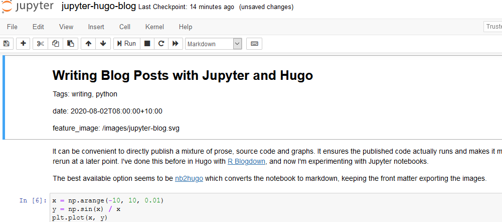
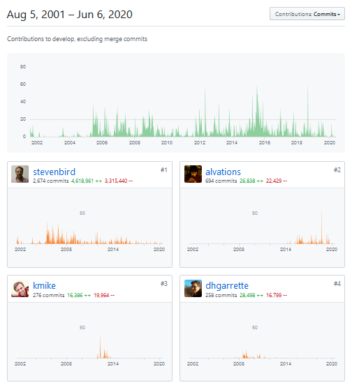
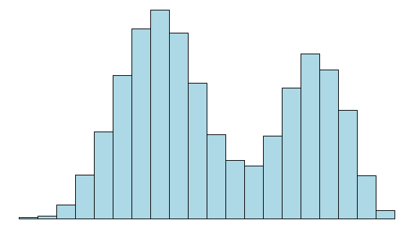
Makemore Subreddits - Part 1 Bigram Model
nlp
makemore
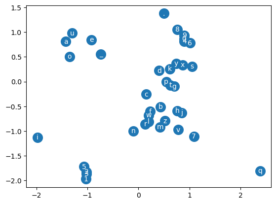
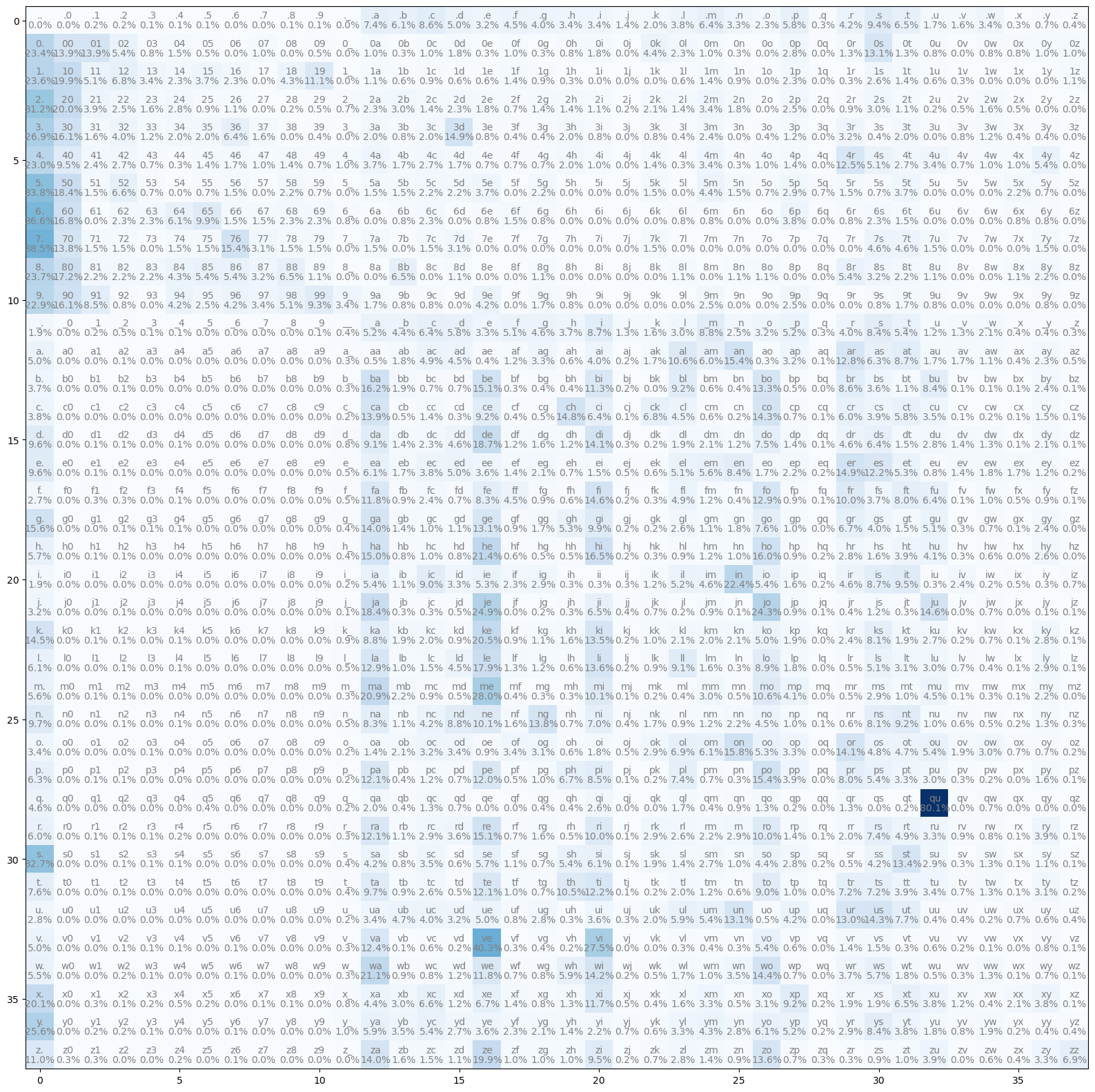
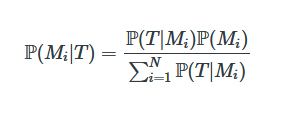
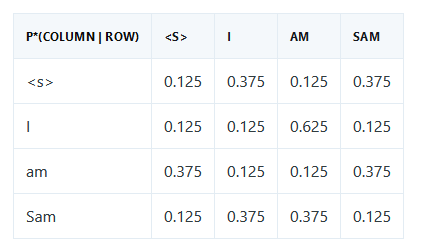
Let’s create a bigram character level language model for subreddit names. This comes at a challenging time when Reddit is changing the terms of its API making most third party apps infeasible (and data extracts like this analysis relies on prohibitively expensive). However the Reddit community has been an interesting place…


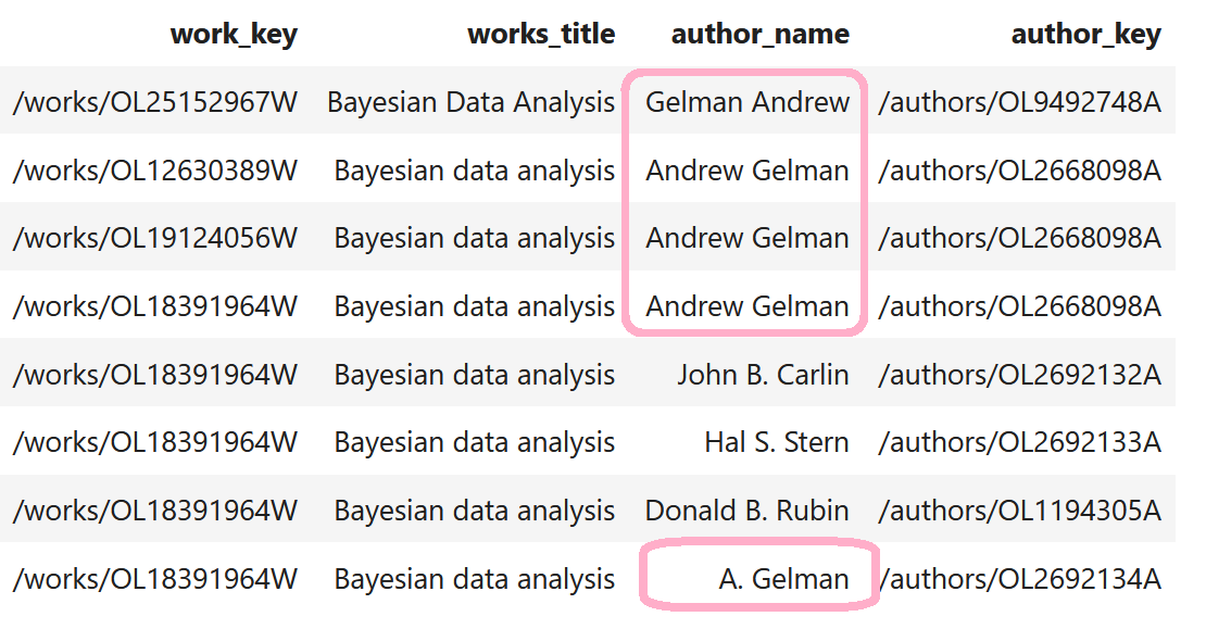
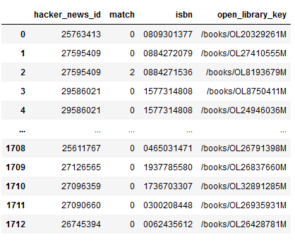
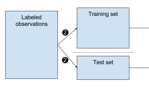
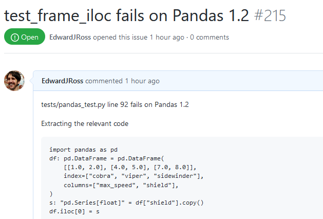
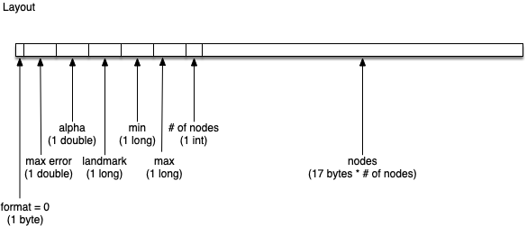
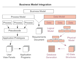
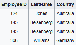
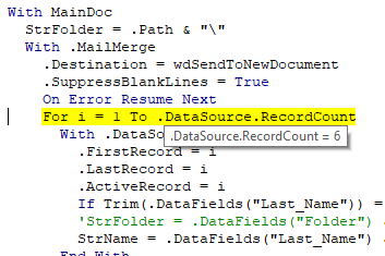
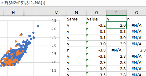
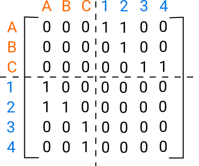
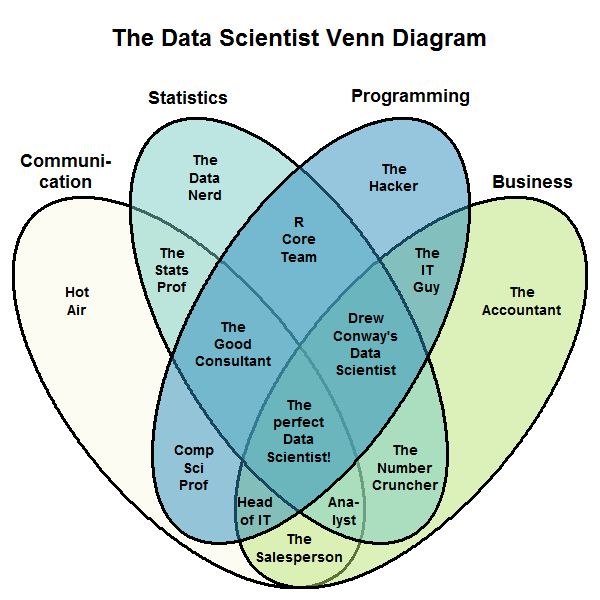
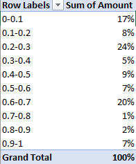
Duplicate Record Detection in Tabular Data
data
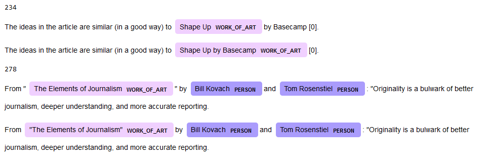
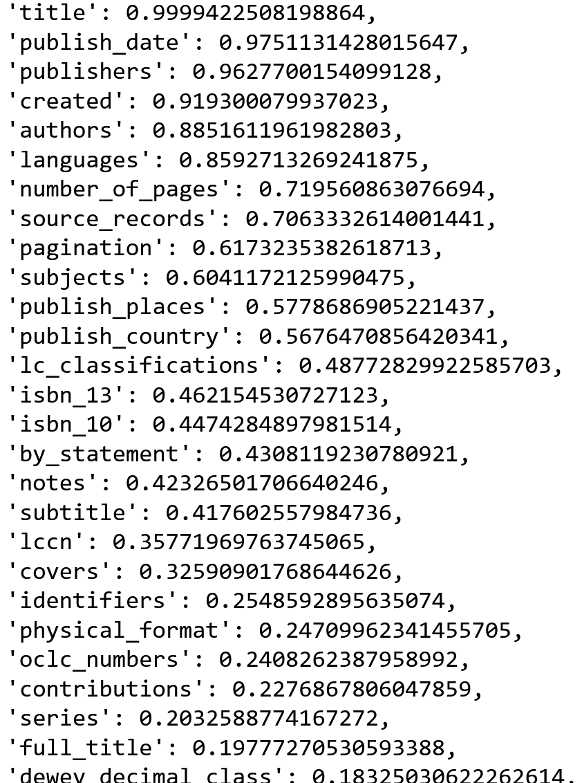
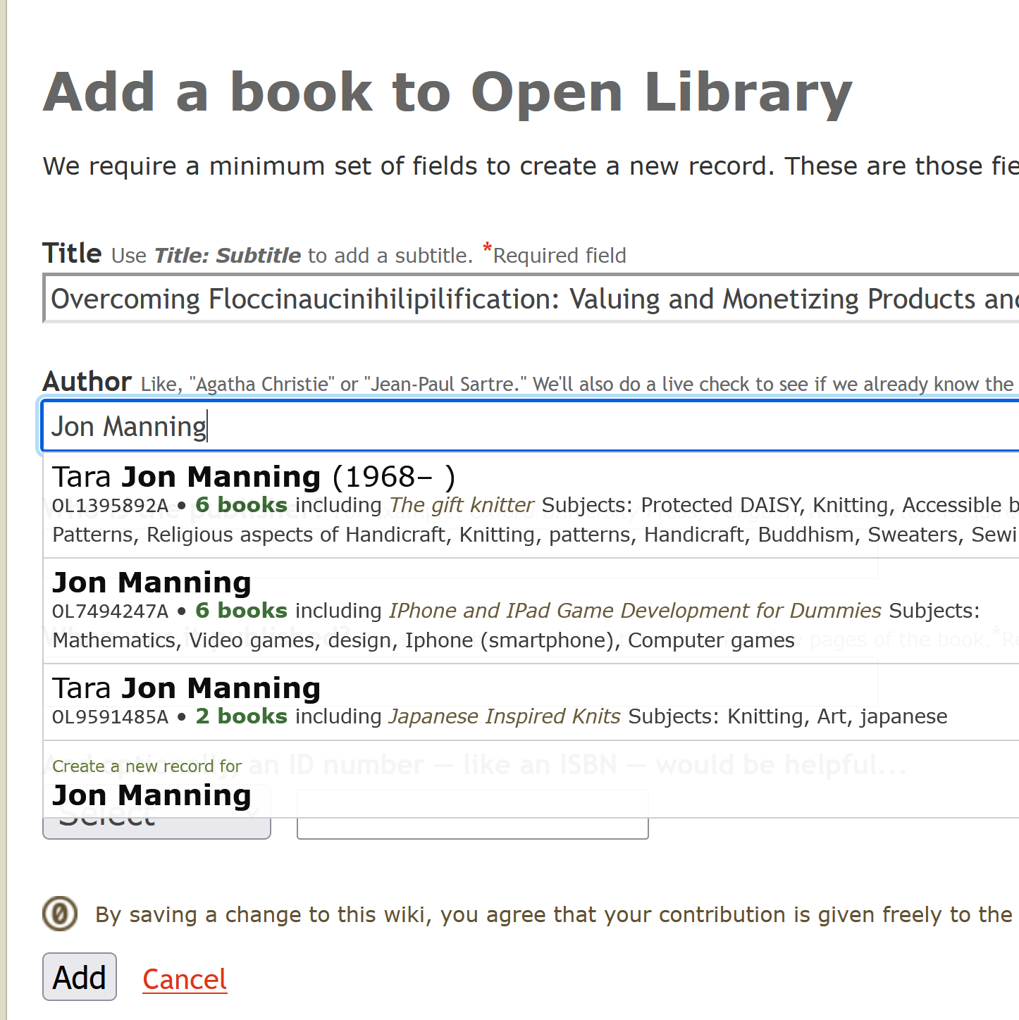
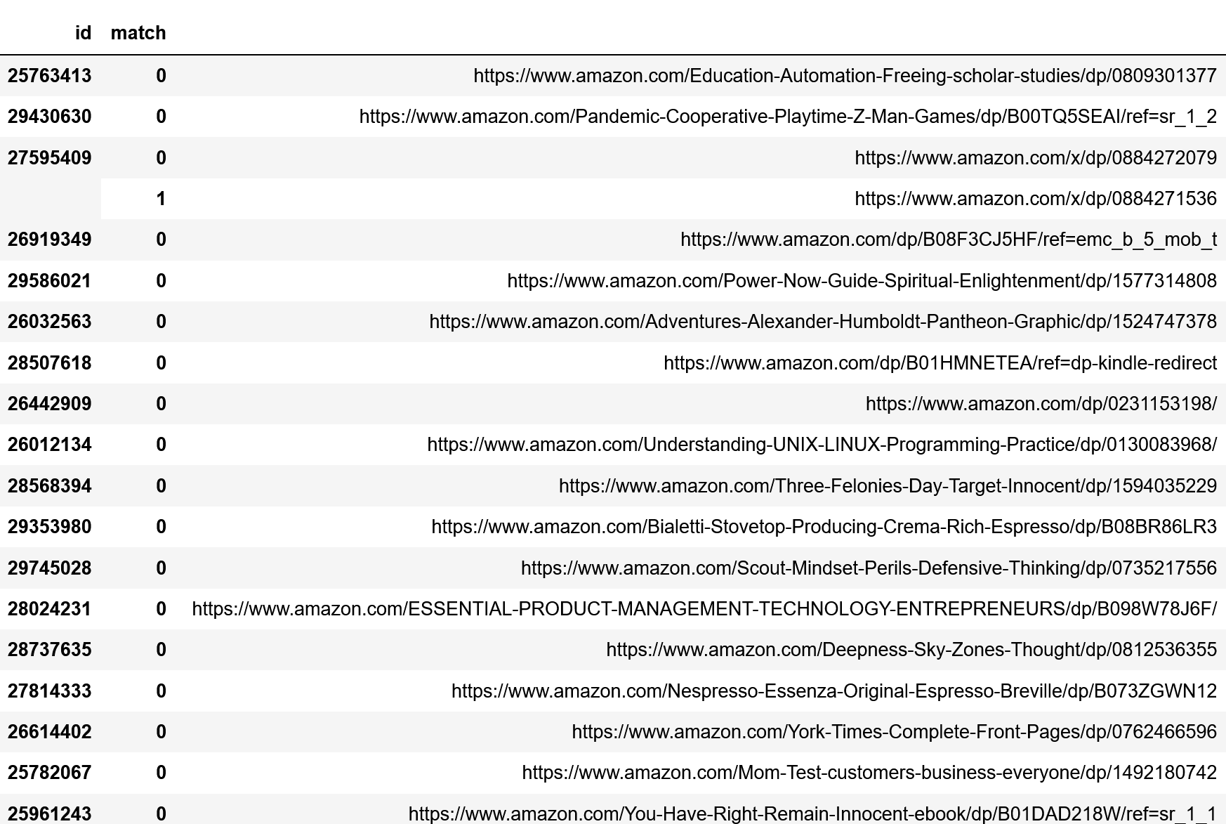
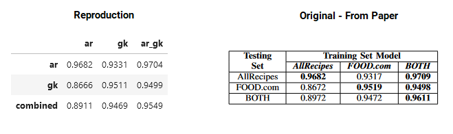
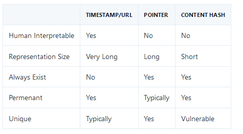
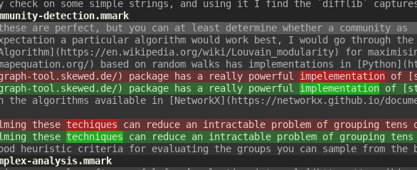
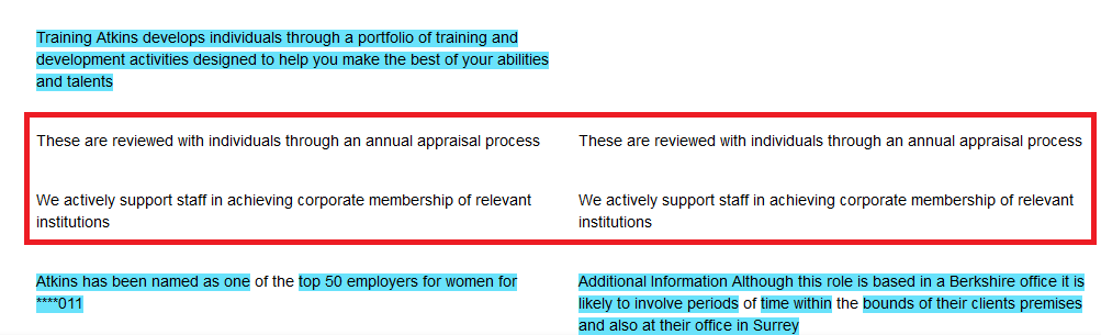
How do you deal with near duplicate data, or join two datasets with some errors? For example when a book is added to Open Library it’s easy for accidental duplicates to occur, and there are many in practice. There are often small differences between duplicates, such as abbreviating author’s names…
![]()


![]()

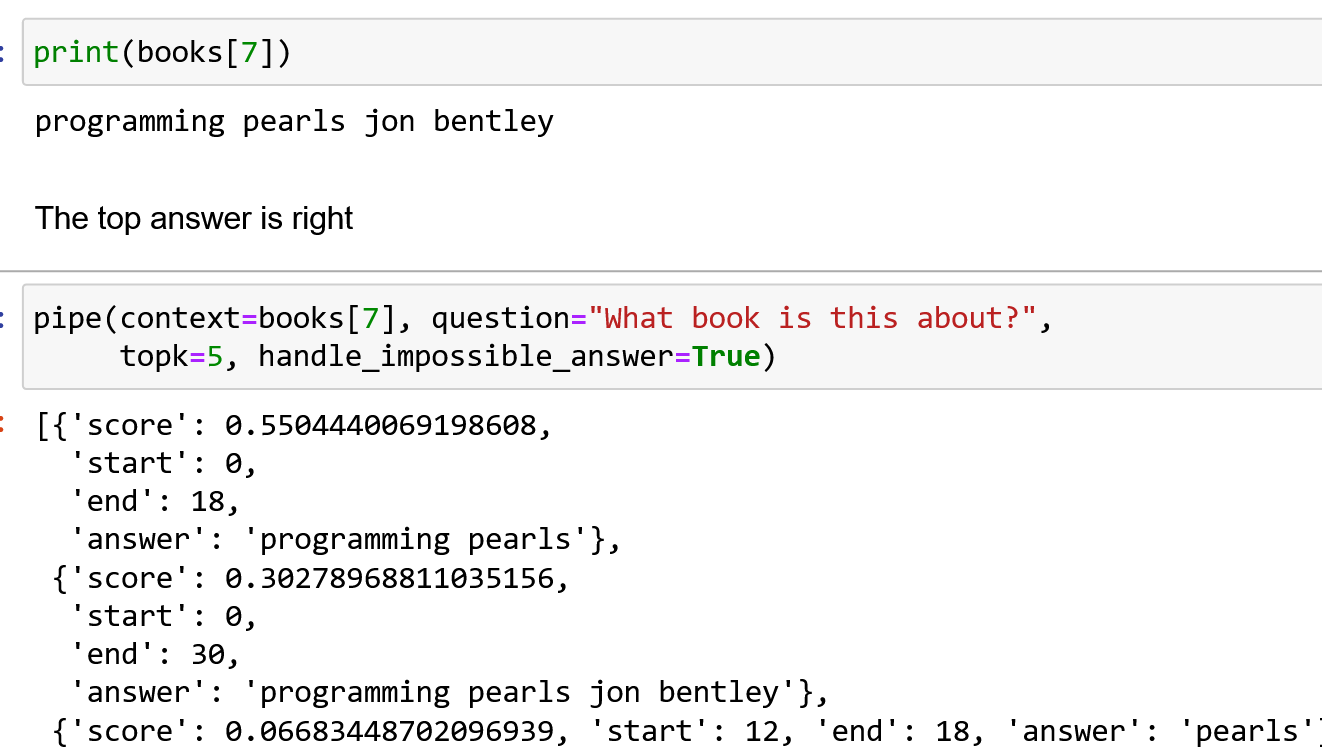
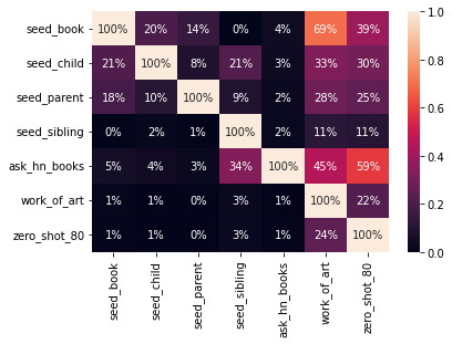
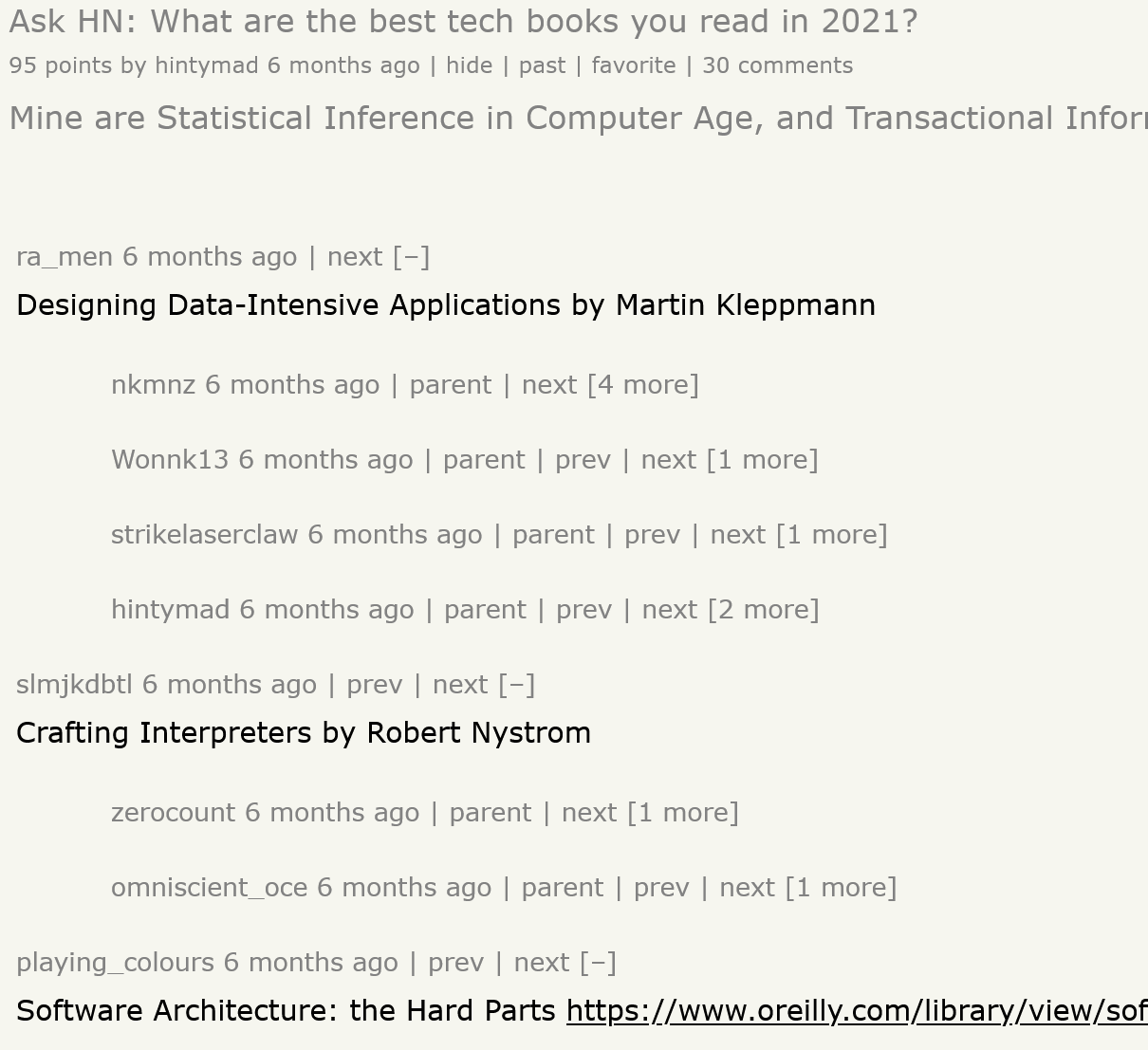
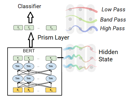
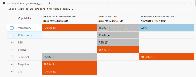
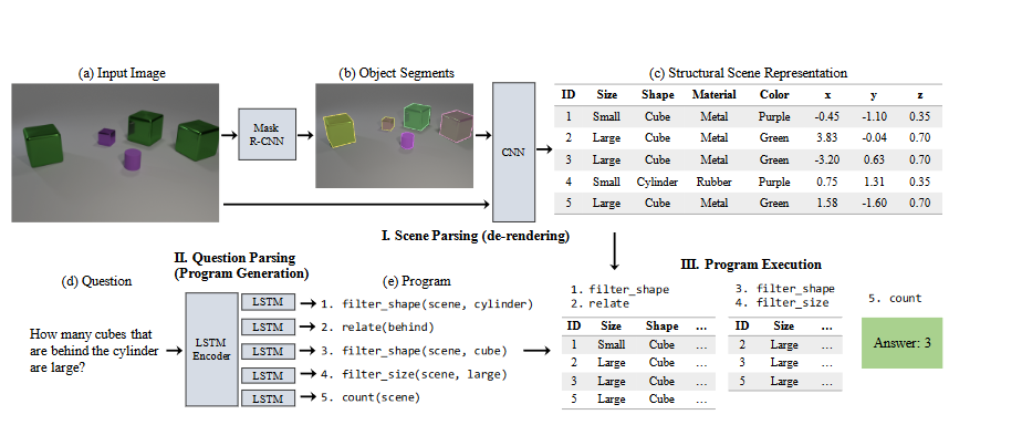
Question Answeeing as Zero Shot NER for Books
nlp
ner
hnbooks
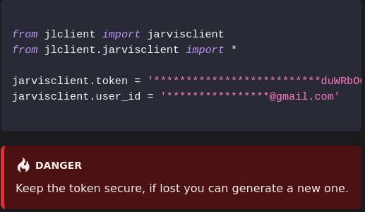
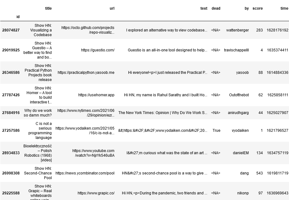
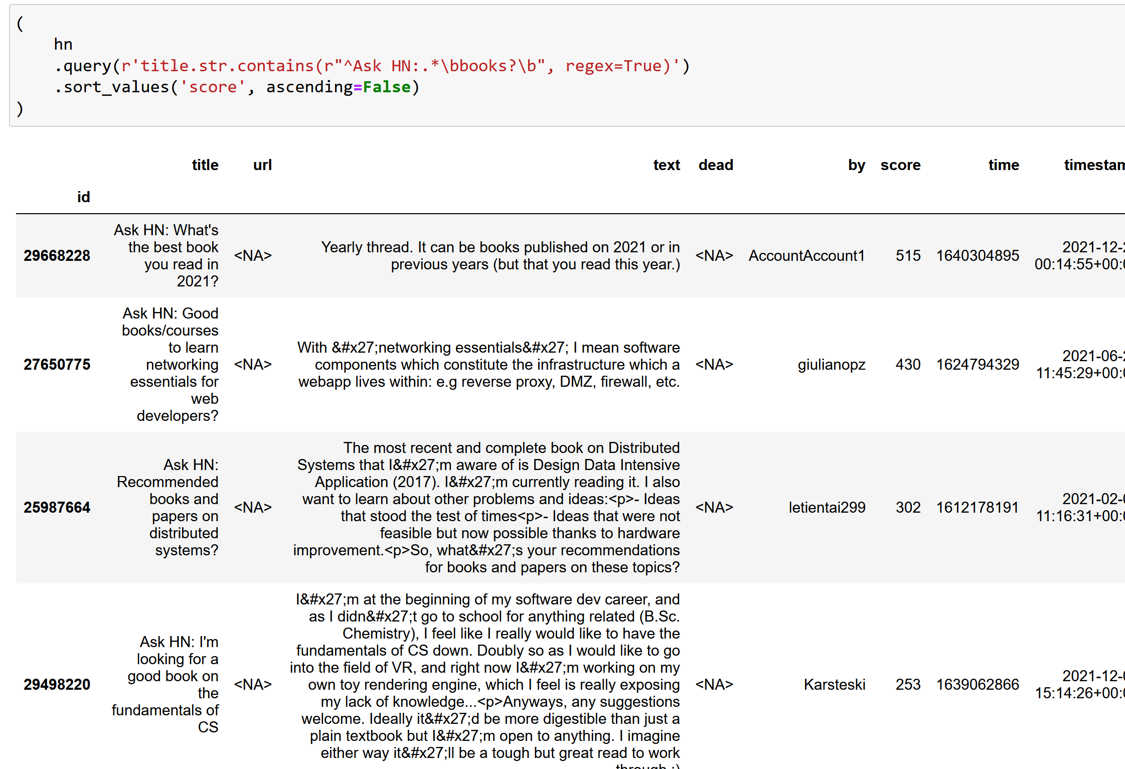
I’m working on a project to extract books from Hacker News. I’ve previously found book recommendations for Ask HN Books, and have used the
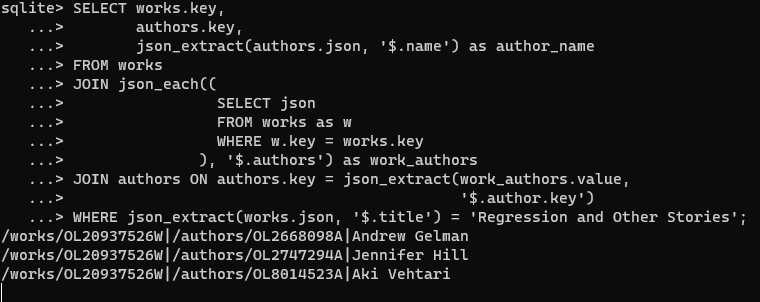
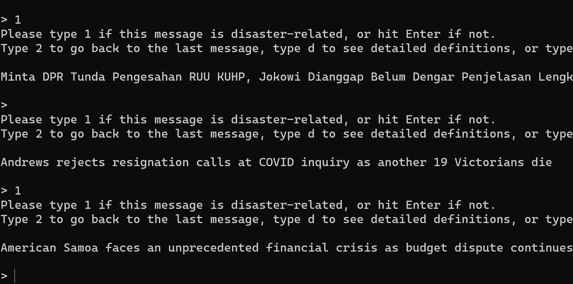
Work of Art named entity from Ontonotes to detect the titles. Another approach is to use extractive question answering as a sort of zero-shot NER. This works amazingly well, at least…
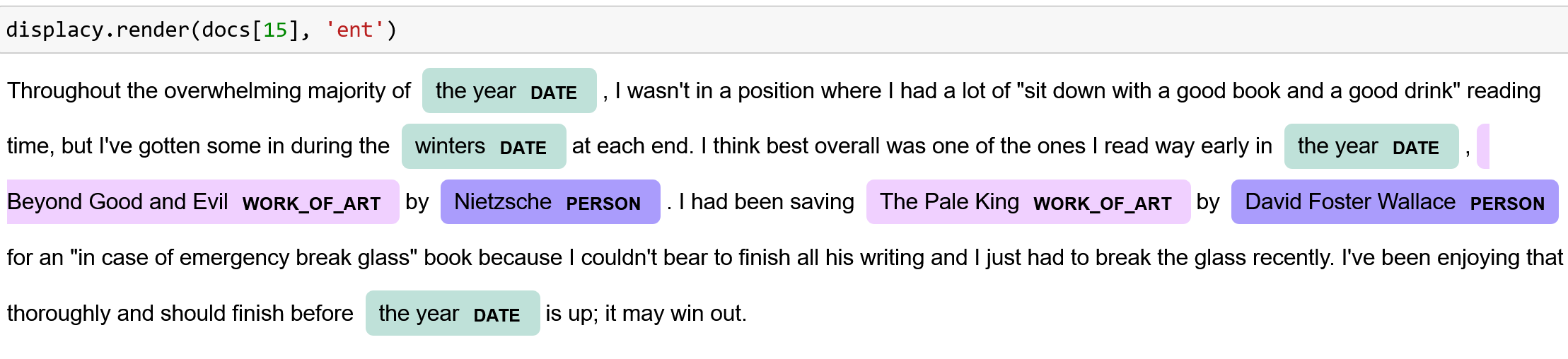
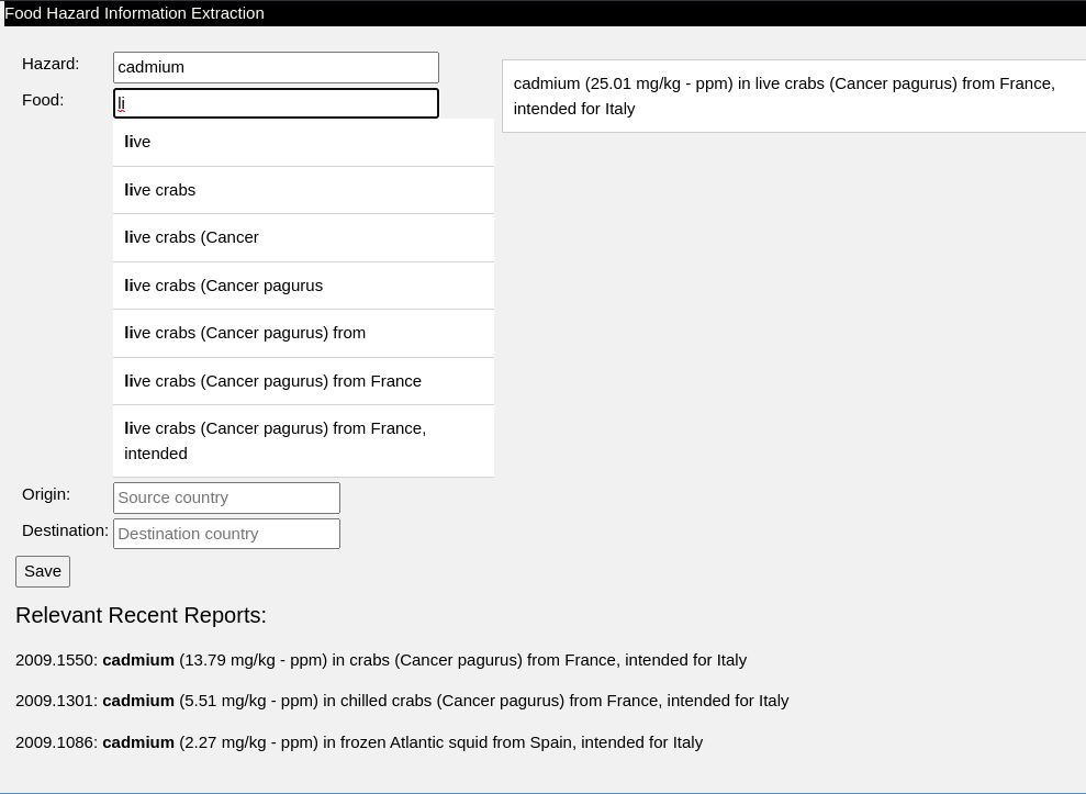
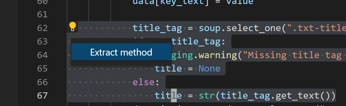
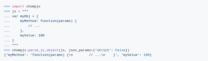
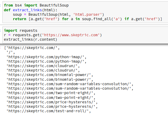
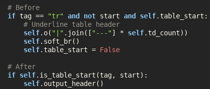
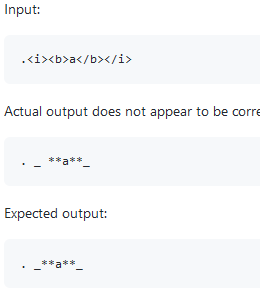
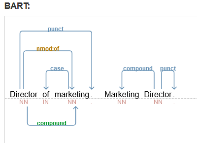
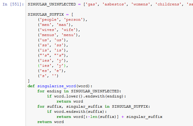
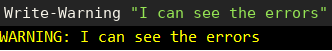
Source Map HTML Tags in Python
python
html
data
nlp
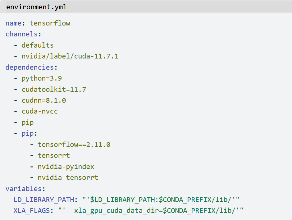
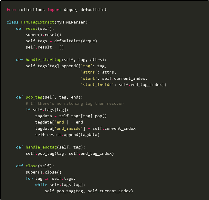
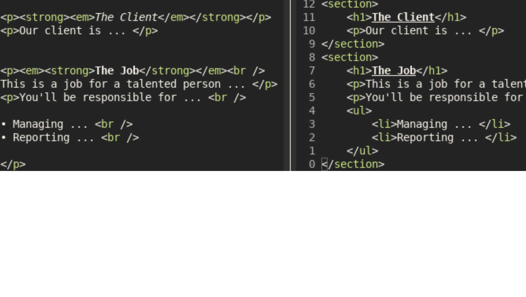
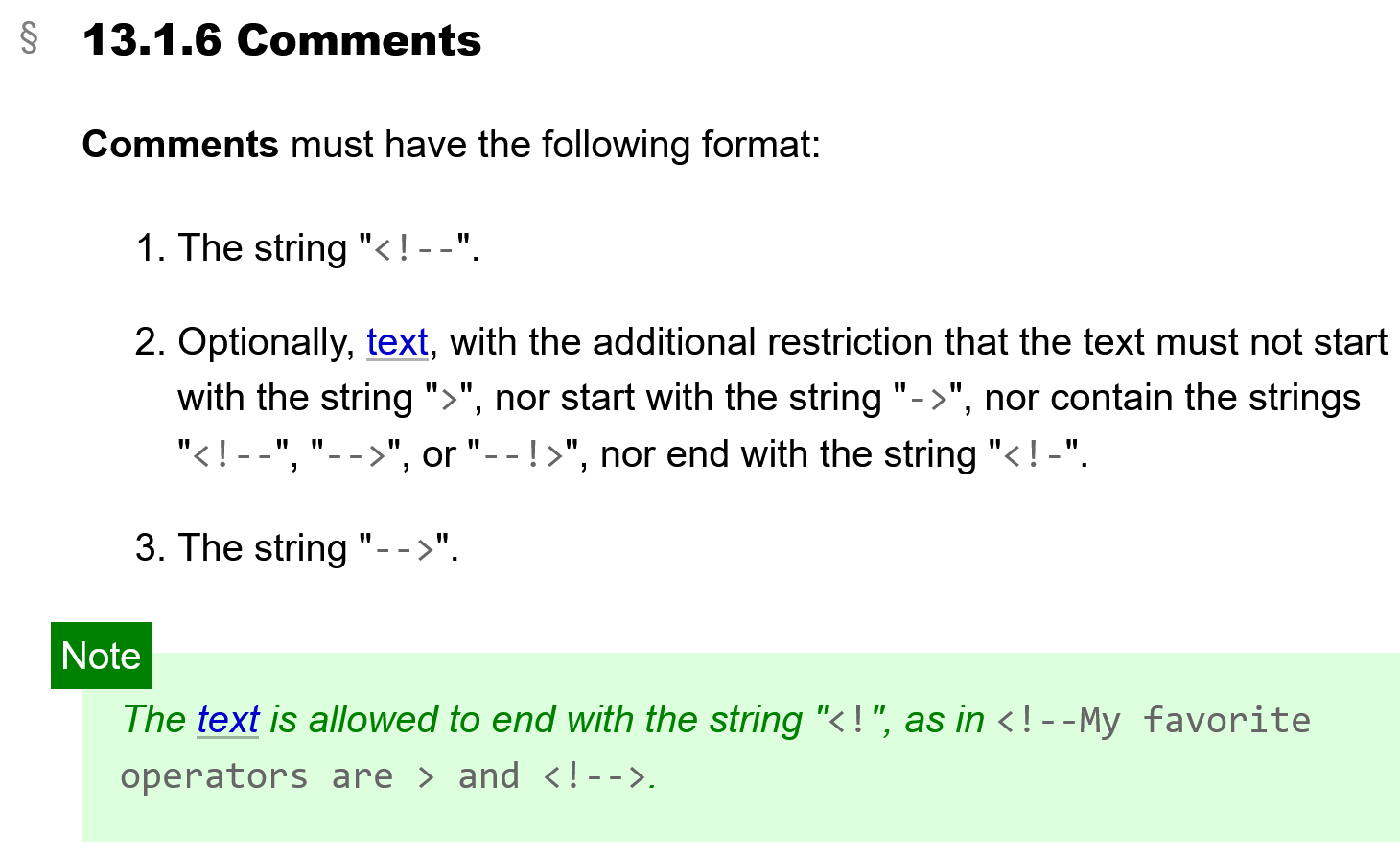
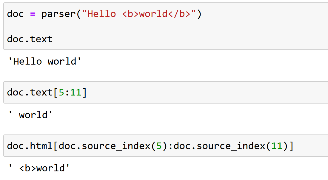
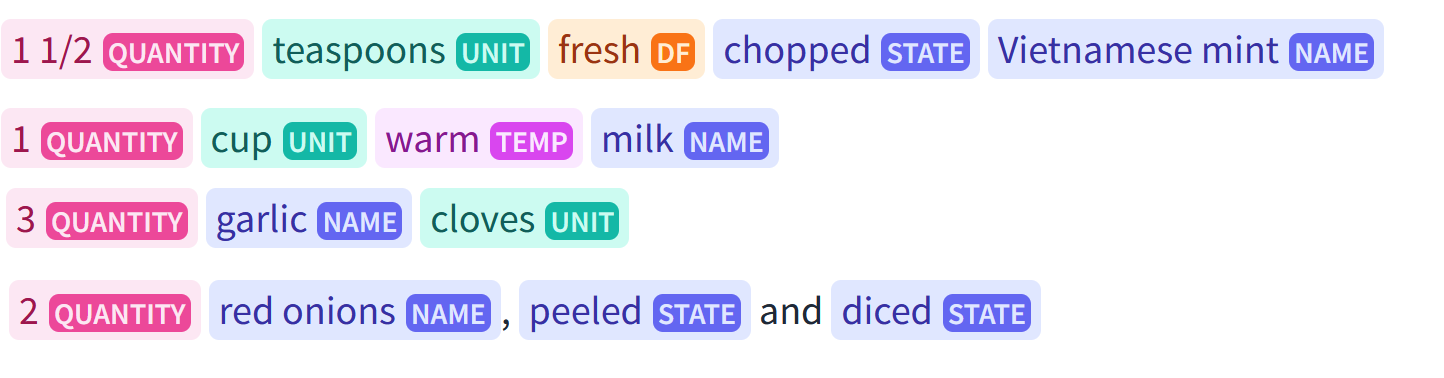
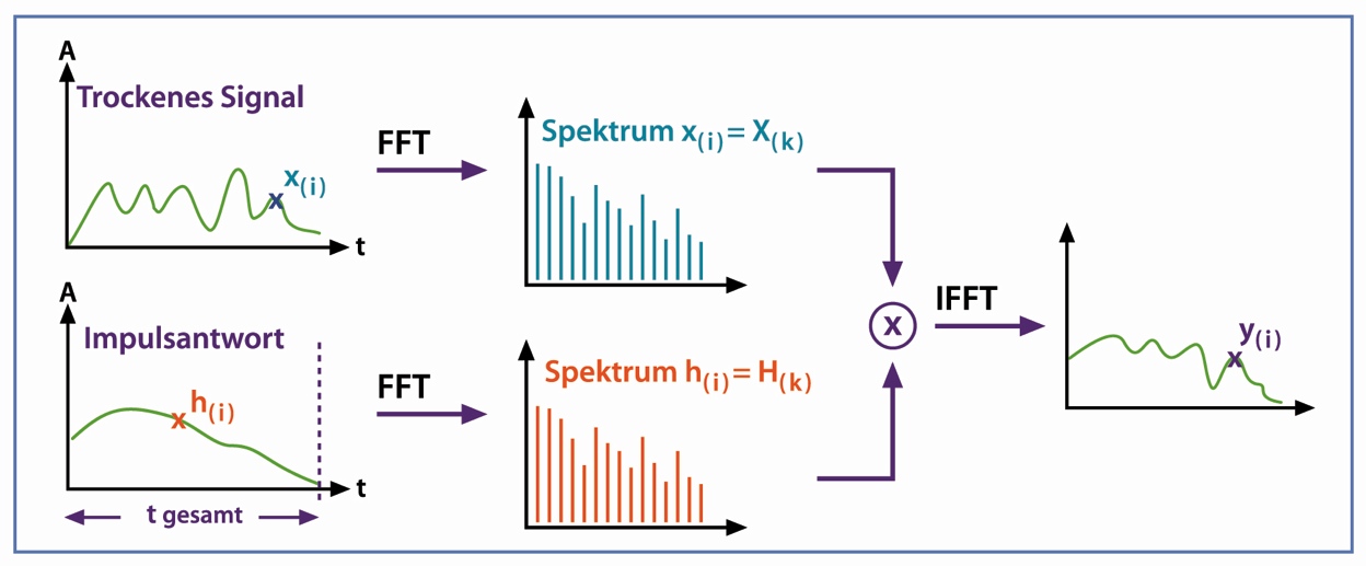
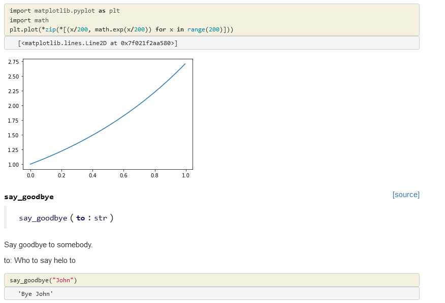
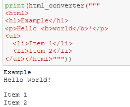
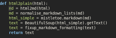
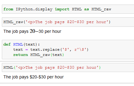
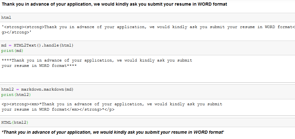
When using NLP in HTML it’s useful to extract the HTML tags which change the meaning of the text. I’ve already shown how to source map the text of HTML using Python’s inbuild HTMLParser. We’ll now adapt this to the task of getting the tags, which could be…
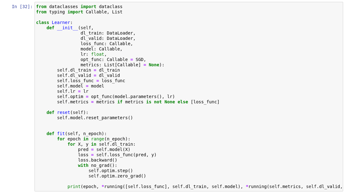
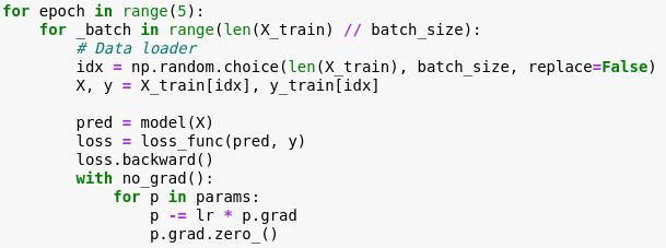
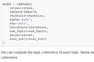
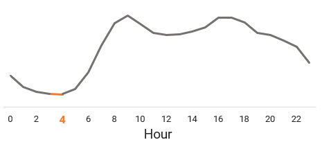
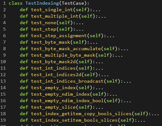
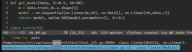
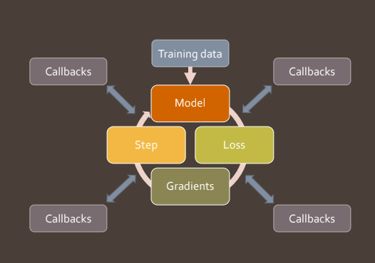
Building a layered API with Fashion MNIST
python
data
fastai
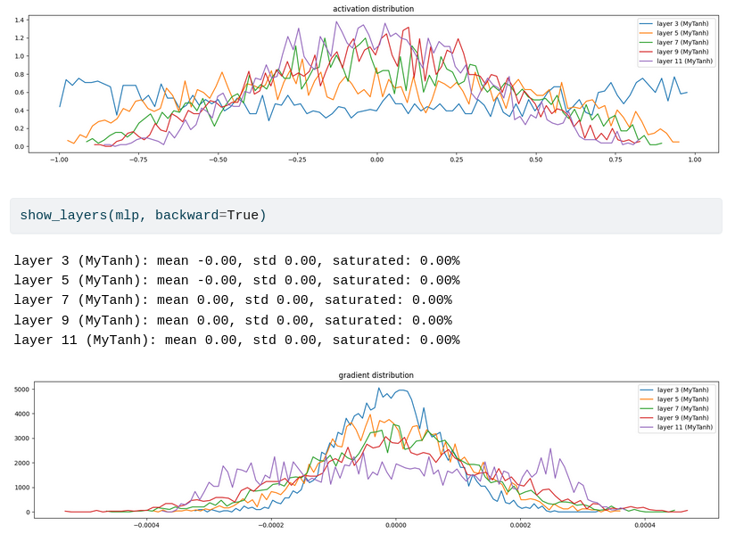
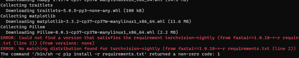
We’re going to build up a simple Deep Learning API inspired by fastai on Fashion MNIST from scratch. Humans can only fit so many things in their head at once (somewhere between 3 and 7); trying to grasp all the details of the training loop at…


![]()


![]()
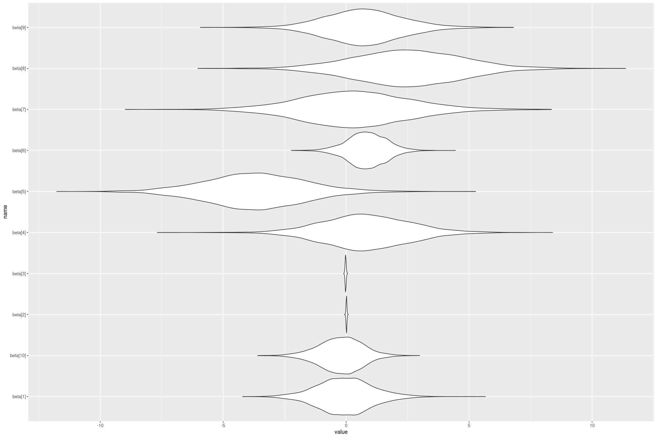
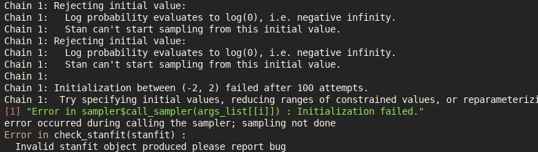
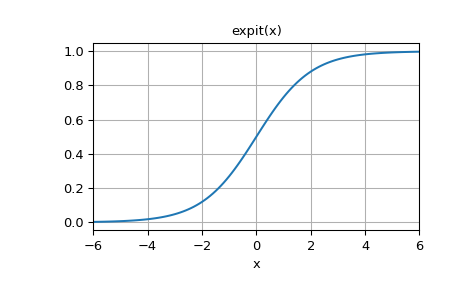
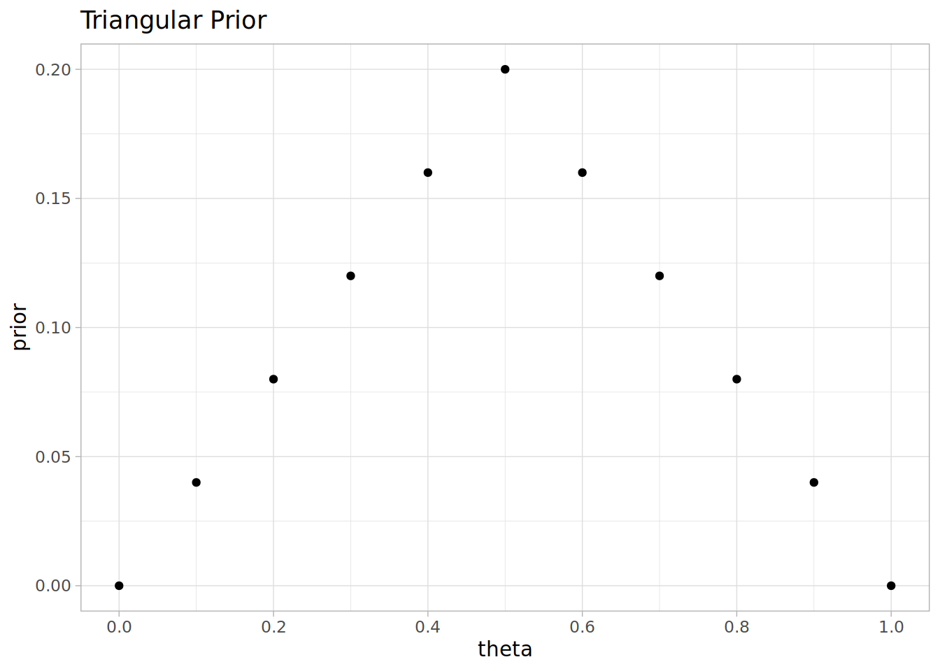
Stan Linear Priors
stan
r
data
statistics
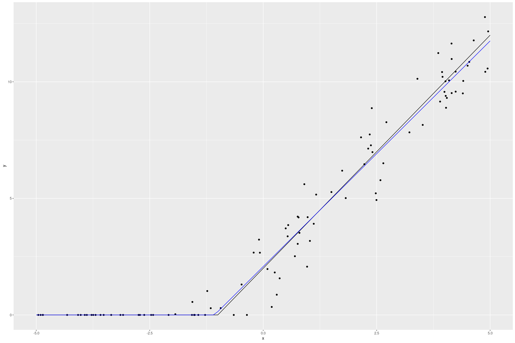
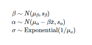
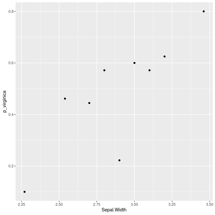
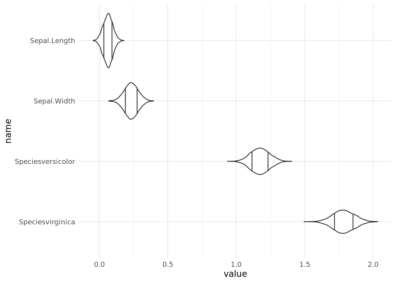
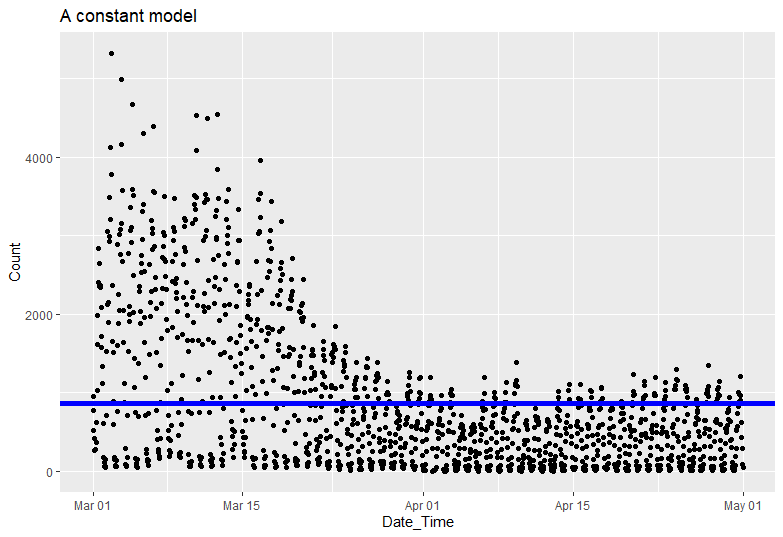
This is the second on a series of articles showing the basics of building models in Stan and accessing them in R. In the previous article I showed how to specify a simple linear model with flat priors in Stan, and fit it in R with a formula syntax. In this article we extend this to specify priors; defaulting…


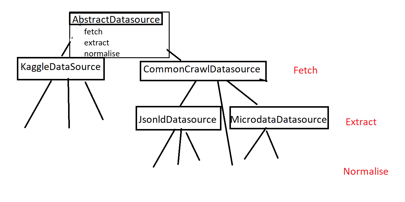
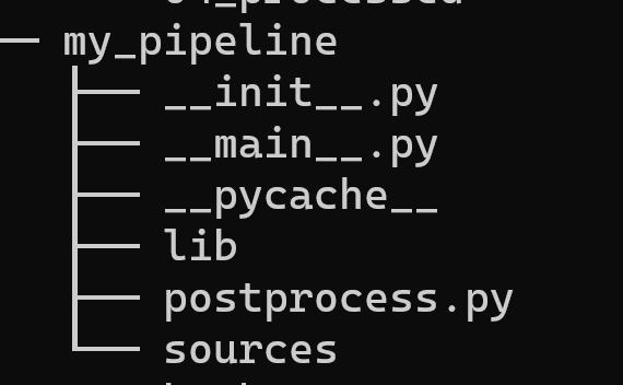
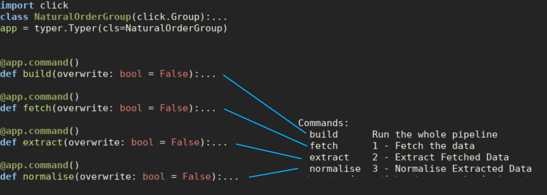
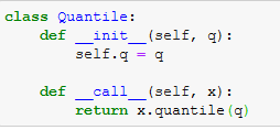
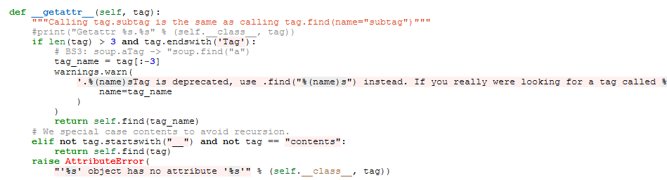
Composition Over Inheritence
programming
jobs
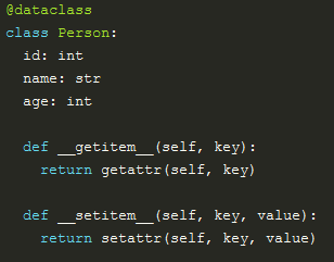
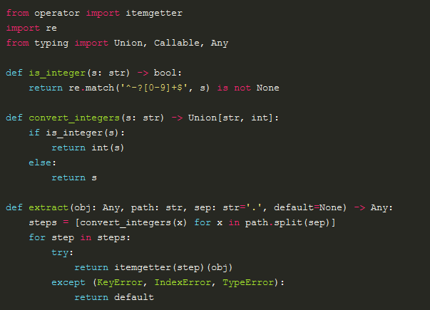
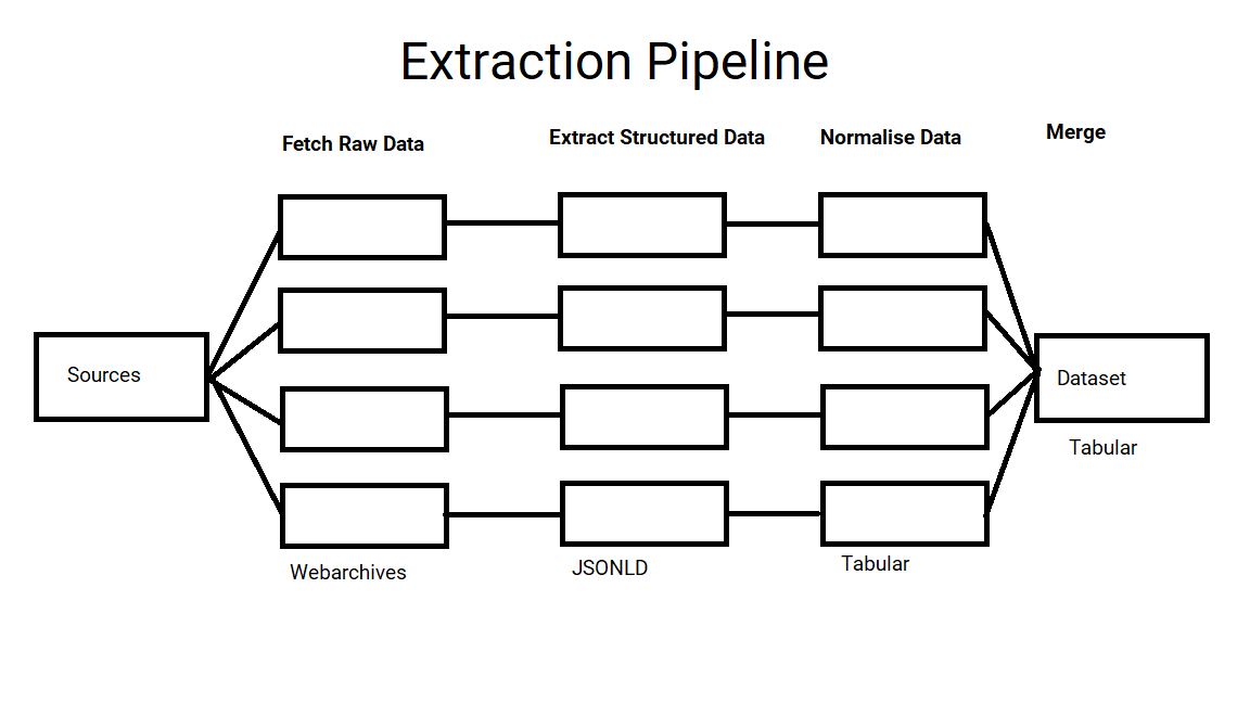
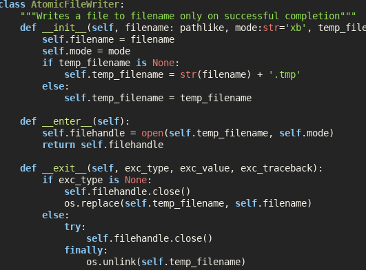
I have been trying to extract job ads from Common Crawl, and have designed a pipeline with 3 phases; fetching the data, extracting the content and normalising the data. However the way I implemented this is using inheritance to remove some of the duplication…

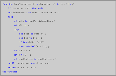
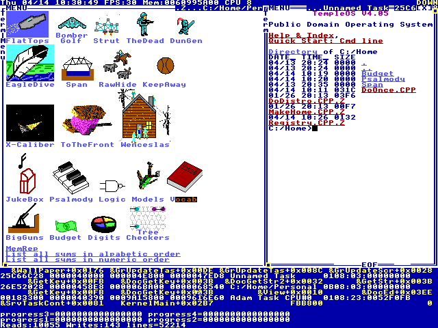
Code Optimisation as a Trade Off
programming
I’ve been writing some ARM Assembly as part of a Raspberry Pi Operating System Tutorial, and writing in Assembly really forces me to think about performance in terms of registers and instructions. When I’m writing Python trying to write concise code leads to…

Hardware Is Hard
programming
I’ve been revisiting baremetal Raspberry Pi programming (with Alex Chadwick’s Baking Pi tutorial, although there are plenty of others). It really highlights how much I take for granted. I spend a lot of time in languages like Python and R processing data, without much understanding of the interpreters…


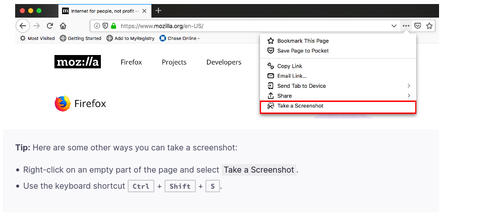
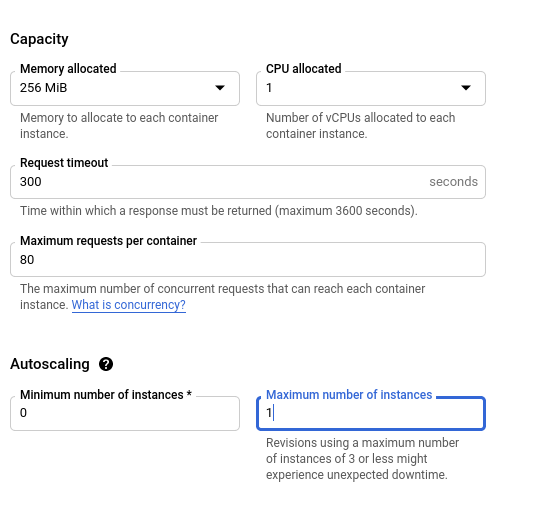
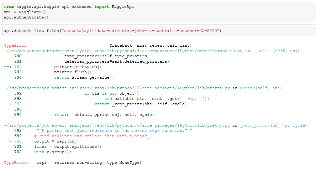
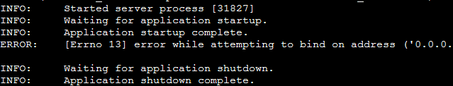
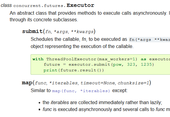
Machine Learning Serving on Google CloudRun
python
I sometimes build hobby machine learning APIs that I want to show off, like whatcar.xyz. Ideally I want these to be cheap and low maintenance; I want them to be available most of the time but I don’t want to spend much time or money maintaining them and I can…

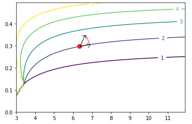
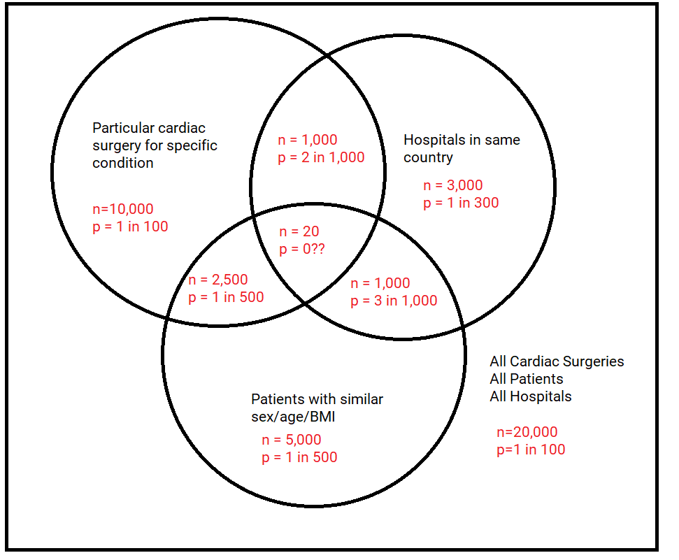
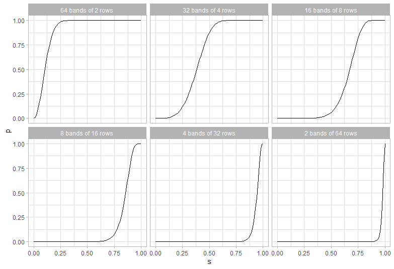
More Profitable A/B with Test and Roll
data
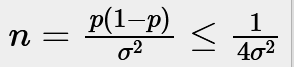
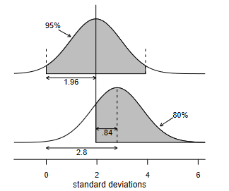
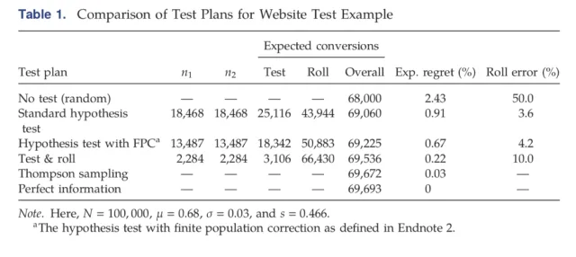
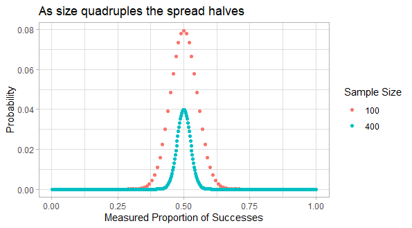
When running an A/B test the sample sizes can seem insane. For example to observe a 2 percentage point uplift on a 60% conversion rate requires over 9,000 people in each group to get the standard 95% confidence level with 80% power. If you’ve only got less than 18,000 customers you can reach, which is very common in businesss to business…

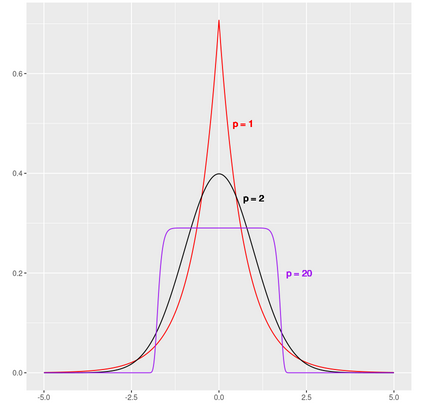
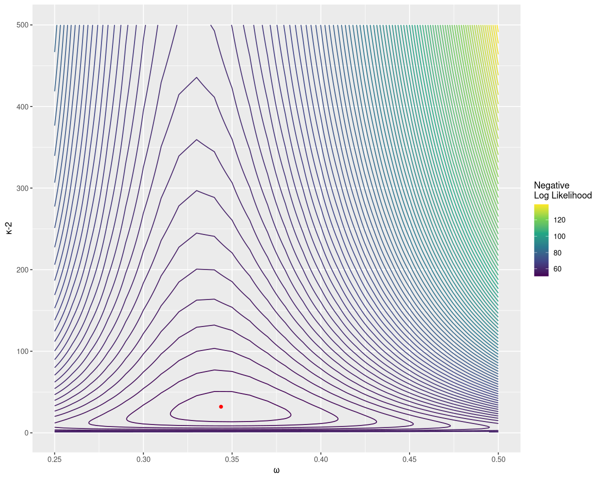
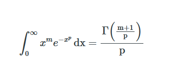
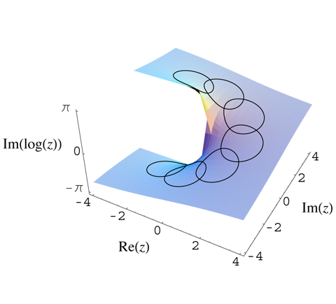
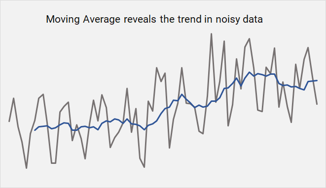
Probability Distributions Between the Mean and the Median
maths
data
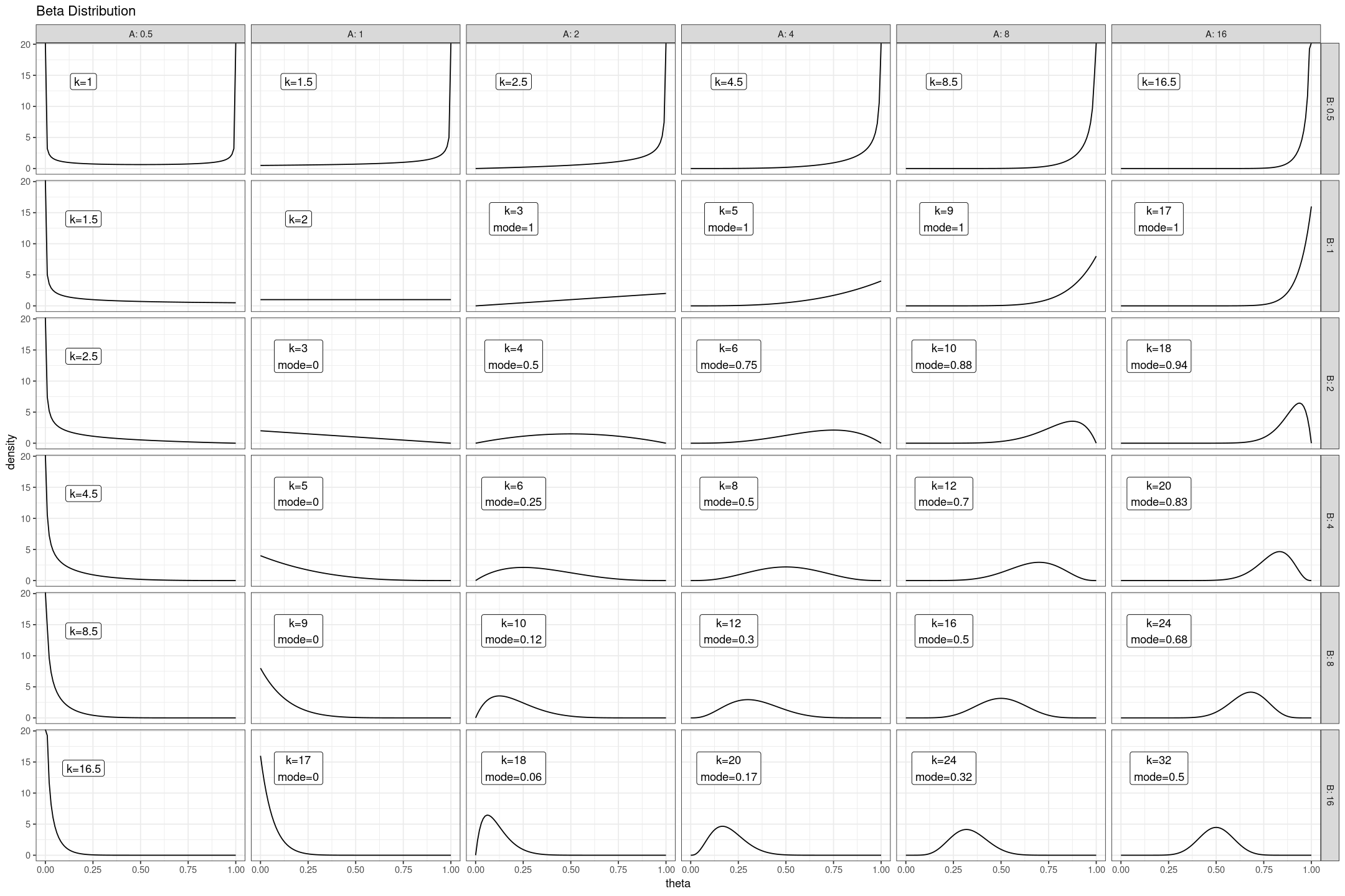
The normal distribution is used throughout statistics, because of the Central Limit Theorem it occurs in many applications, but also because it’s computationally convenient. The expectation value of the normal distribution is the mean, which has many nice…

![]()


The Righteous Mind: Book Review
books
Johnathan Haidt’s The Righeous Mind: Why Good People are Divided by Politics and Religion is about the moral norms of groups. As someone not familiar with moral psychology I found the book discussed many interesting ideas I wasn’t aware of, but didn’t provide much evidence for…

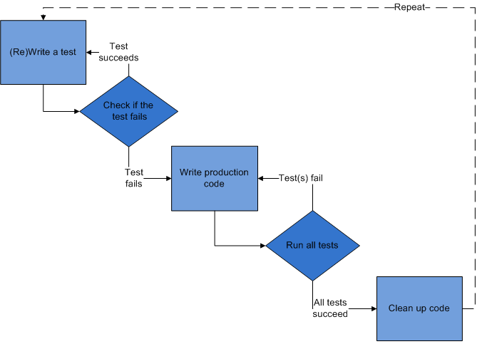
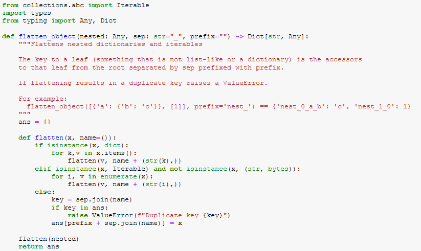
What Is a Better Programming Approach?
programming
When you solve a problem in code you will use some programming approach, and the approach you choose can make a big impact on your efficiency. I talk about approach rather than language because it’s more than just the language. A project will typically only use a subset of the language (especially for massive languages like C++), some…


Truly Independent Thinkers
general
I was reading [Paul Graham’s How to Think For Yourself] where he talks about independent-mindedness. His examples are scientists, investors, startup founders and essayists as professions where you can’t do well without thinking differently from your peers. While there’s…

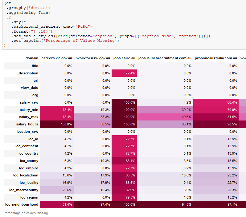
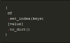
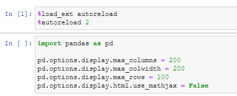
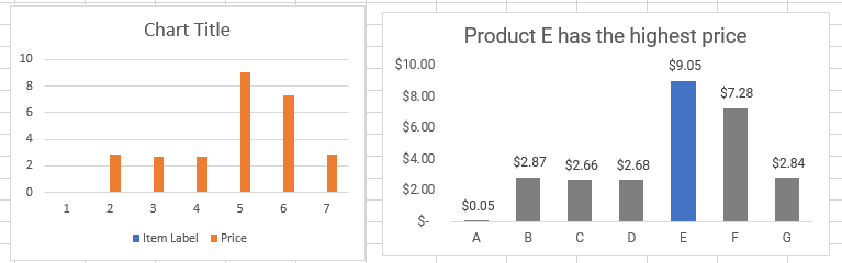
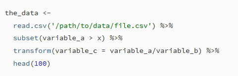
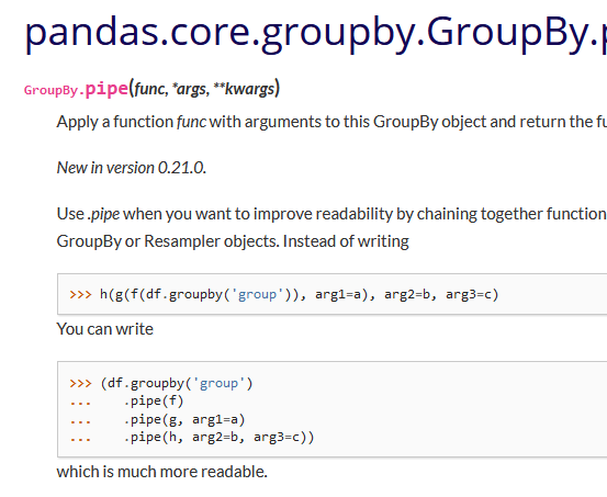
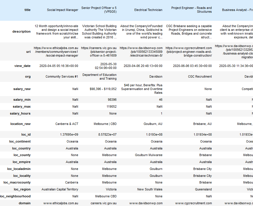
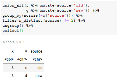
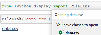
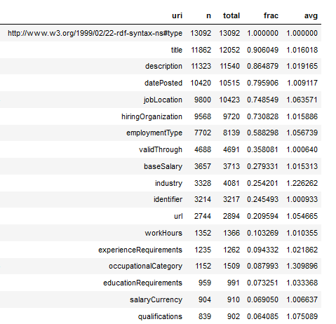
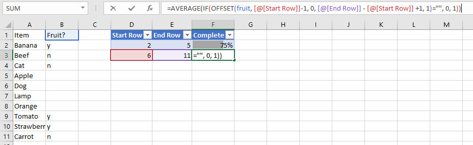
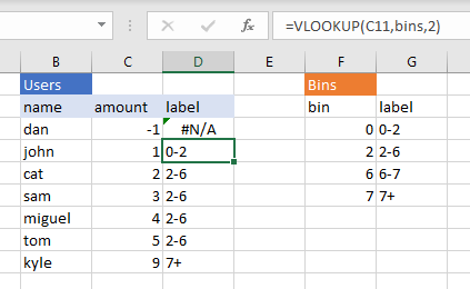
Decorating Pandas Tables
python
data
pandas
jupyter
When looking at Pandas dataframes in a Jupyter notebook it can be hard to find what…


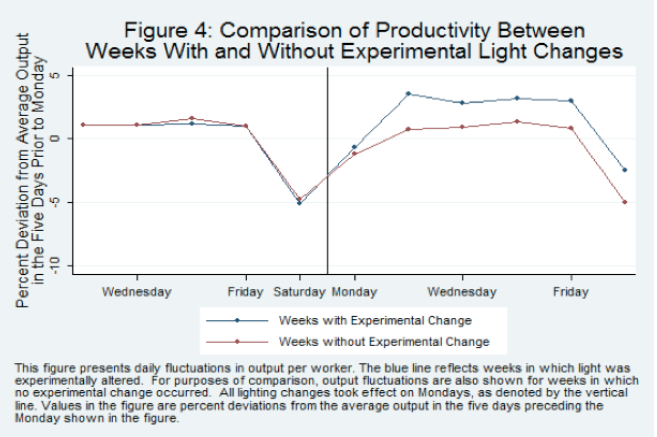
Myth of the Hawthorne Effect
general
The Hawthorne effect is where when measuring the effect of lighting changes on worker output in an electrical factory any change increased output, even back to the original lighting conditions. I’ve heard this explained as running the experiment caused the employees to be observed more closely…
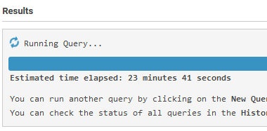
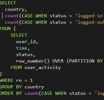
Running out of Resources on AWS Athena
athena
presto
AWS Athena is a managed version of Presto, a distributed database. It’s very convenient to be able to run SQL queries on large datasets, such as Common Crawl’s Index, without having to deal with managing the infrastructure of big data. However the downside of a managed service is when you hit its limits there’s no way of…


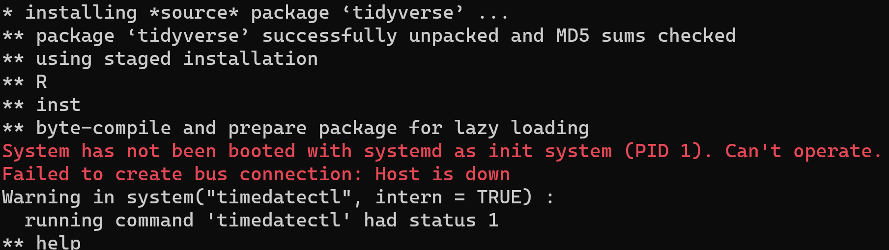
Updating a Python Project: Whatcar
whatcar
python
programming
The hardest part of programming isn’t learning the language itself, it’s getting familiar with the gotchas of the ecosystem. I recently updated my whatcar car classifier in Python after leaving it for a year and hit a few roadblocks along the way. Because I’m familiar with Python I knew enough heuristics to work through them quickly, but it…


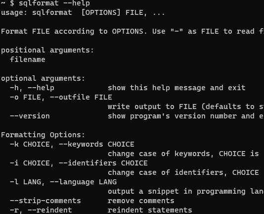
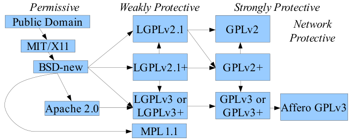
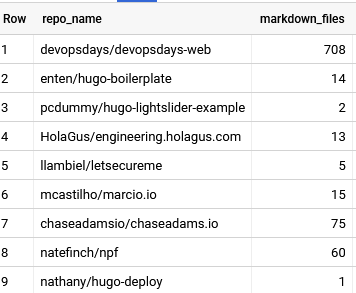
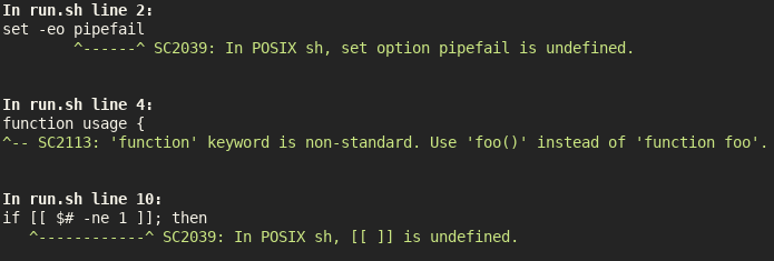
Choosing a Static Site Generator
programming
blog
Static website generators fill a useful niche between handcoding all your HTML and running a server. However there’s a plethora of site generators and it’s hard to choose between them. However I’ve got a simple recommendation: if you’re writing a blog use Jekyll…
![]()


Can I? Must I? Should I?
general
Whenever someone gets an idea in their head they start filtering out evidence that contradicts that idea. This idea is called confirmation bias, people start looking for evidence that confirms their current idea and neglecting evidence that challenges it. There’s no way to completely beat a bias, but something that…
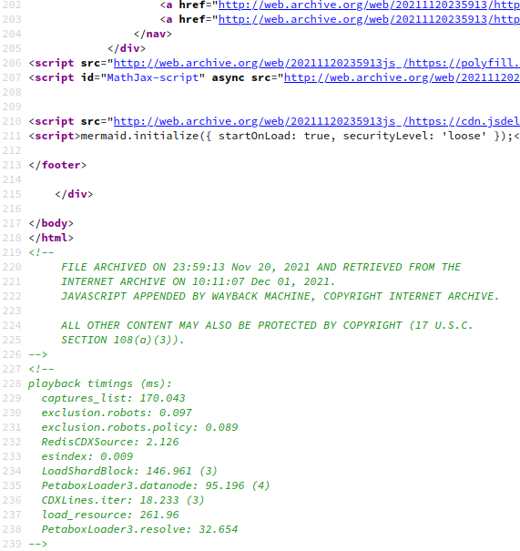
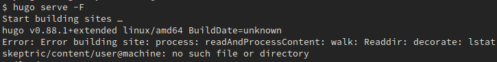
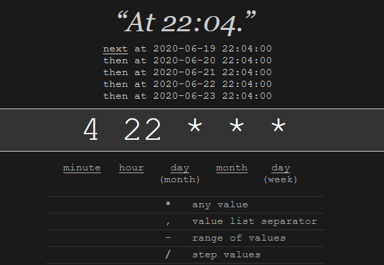
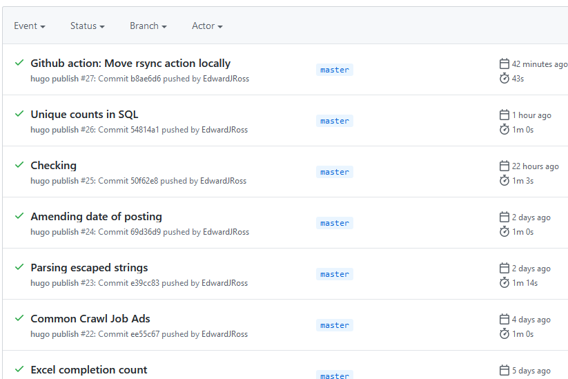
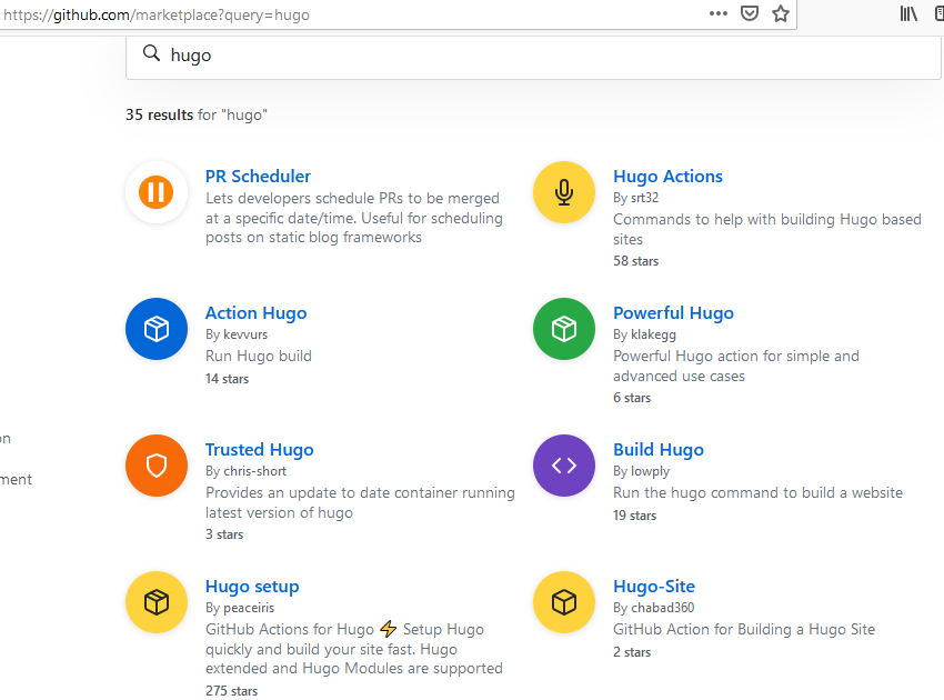
Manually Triggering Github Actions
programming
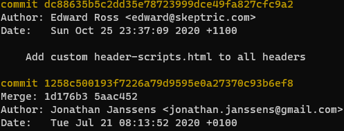
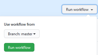
I have been publishing this website using Github Actions with Hugo on push and on a daily schedule. I recently received an error notification via email from Github, and wanted to check whether it was an intermittent error. Unfortunately I couldn’t find anyway to rerun…


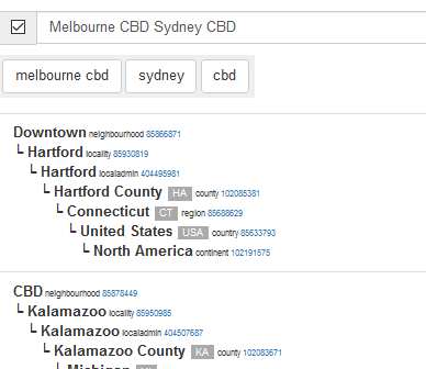
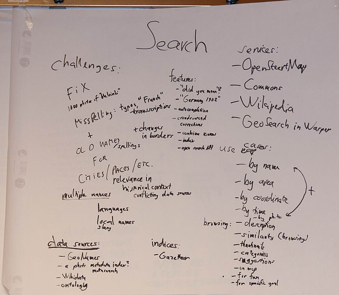
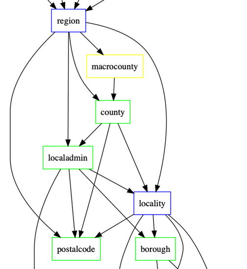
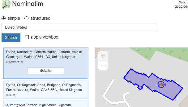
Refining Location with Placeholder
data
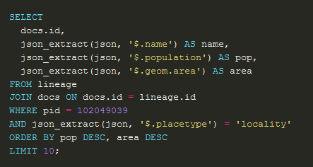
Placeholder is a great library for Coarse Geocoding, and I’m using it for finding locations in Australia. In my application I want to get the location to a similar level of granularity; however the input may be for a higher level of granularity. Placeholder doesn’t directly…


Removing Timezone in Athena
presto
athena
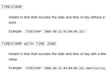
When creating a table in Athena I got the error:
Invalid column type for column: Unsupported Hive type: timestamp with time zone. Unfortunately it can’t support timestamps with timezone. In my case all the data was in UTC so I just needed to remove the timezone to create the table. The easiest way to…


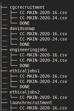
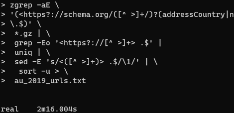
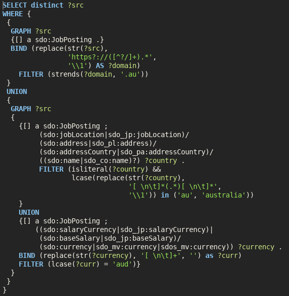
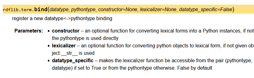
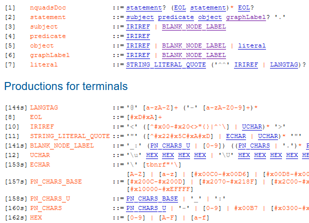
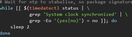
Processing RDF nquads with grep
data
commoncrawl
I am trying to extract Australian Job Postings from Web Data Commons which extracts structured data from Common Crawl. I previously came up with a SPARQL query to extract the Australian jobs from the domain, country and currency. Unfortunately it’s quite slow, but we can speed it up dramatically by replacing it with a…
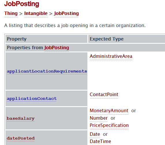

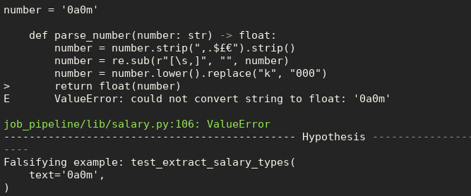
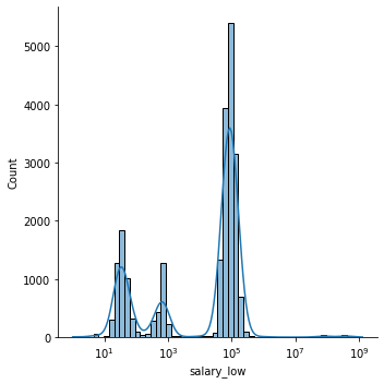
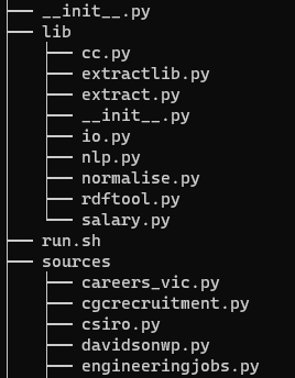
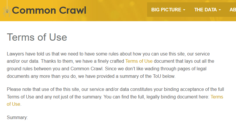
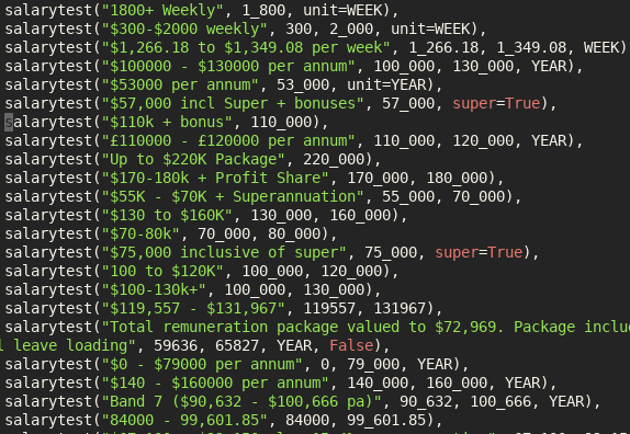
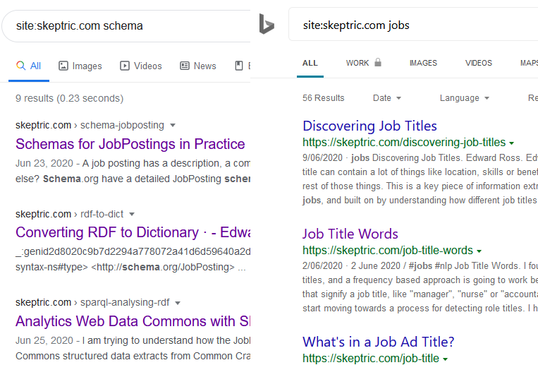
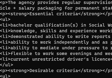
Extracting Job Ads from Common Crawl
commoncrawl
jobs
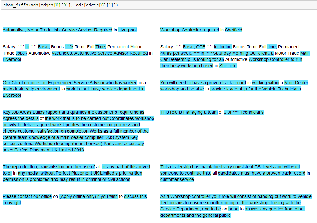
I’ve been using data from the Adzuna Job Salary Predictions Kaggle Competition to extract skills, find near duplicate job ads and understand seniority of job titles. But the dataset has heavily processed ad text which makes it harder to do natural language processing on. Instead I’m going to…
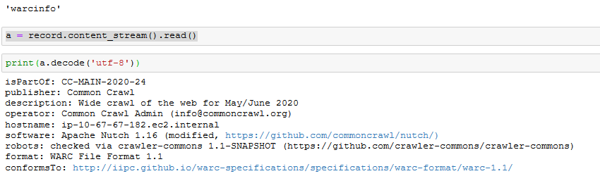
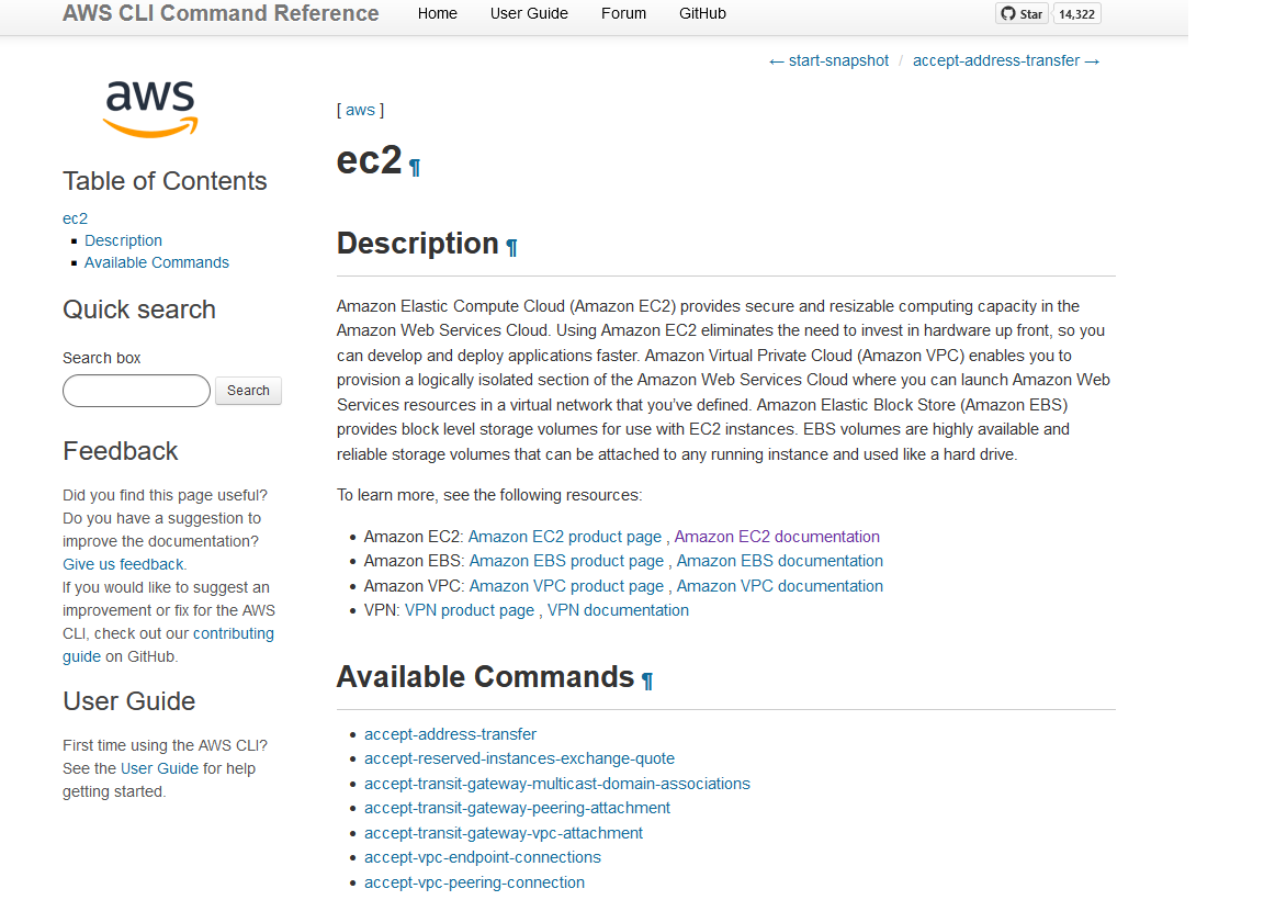
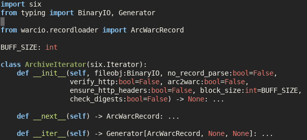
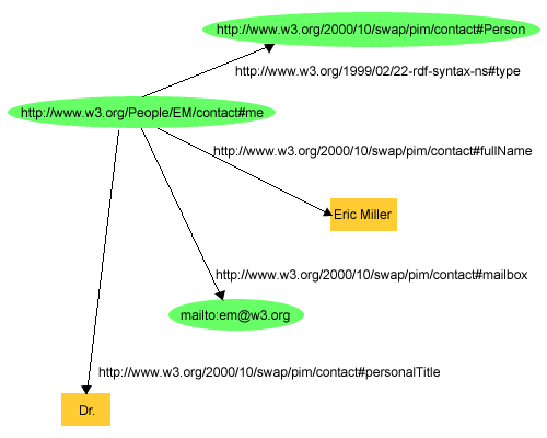
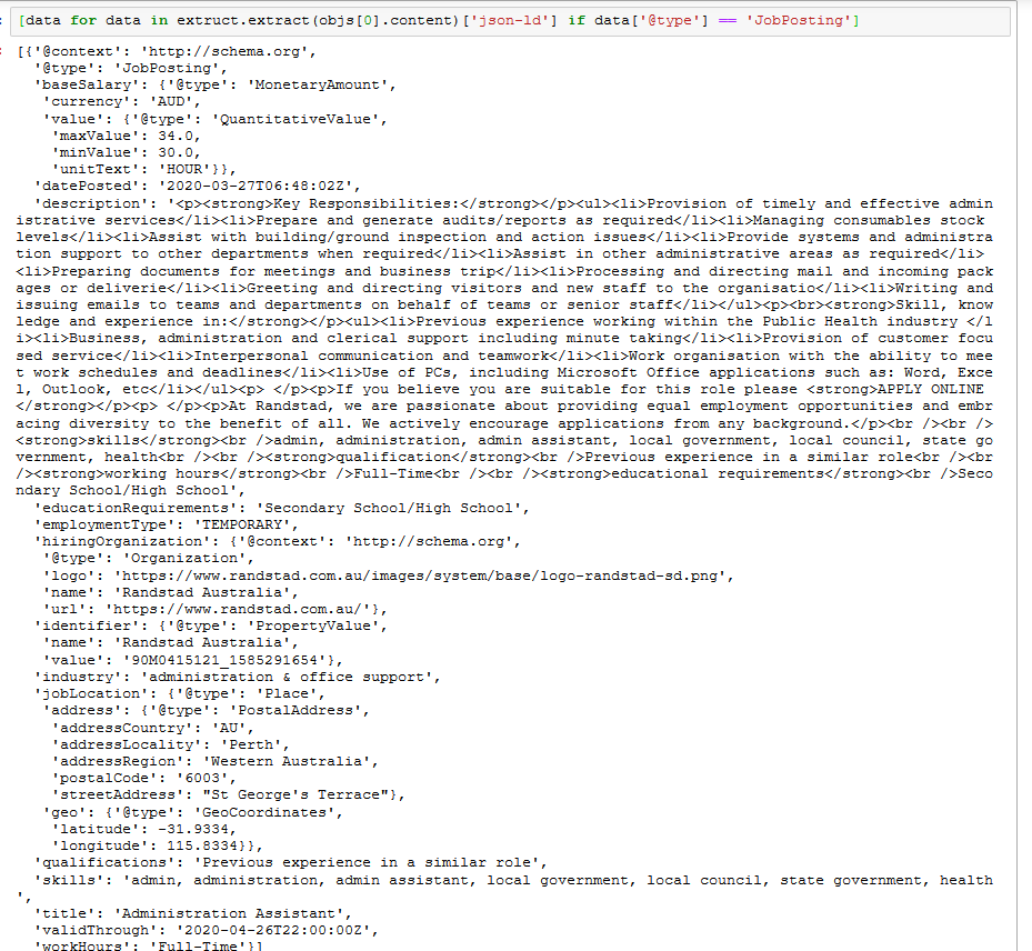
Extracing Text, Metadata and Data from Common Crawl
commoncrawl
data
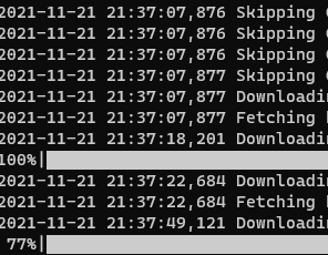
Common Crawl builds an open dataset containing over 100 billion unique items downloaded from the internet. You can search the index to find where pages from a particular website are archived, but you still need a way to access the…
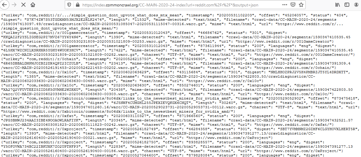
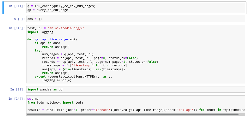
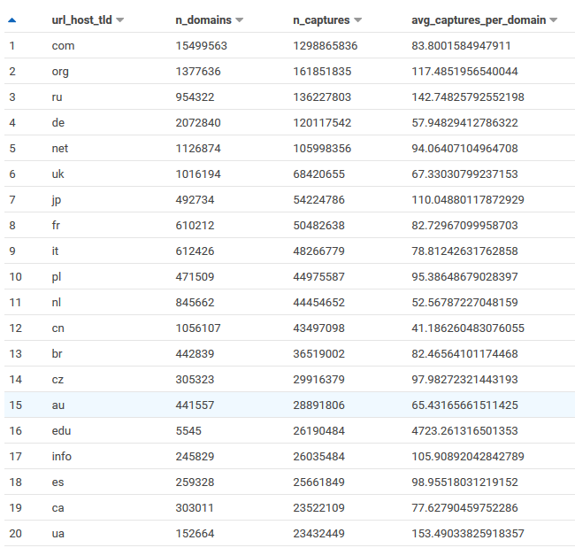
Searching 100 Billion Webpages Pages With Capture Index
commoncrawl
data
Common Crawl builds an open dataset containing over 100 billion unique items downloaded from the internet. Every month they use Apache Nutch to follow links accross the web and download over a billion unique items to Amazon S3, and have data back to 2008. This is like what Google and Bing do to build their…
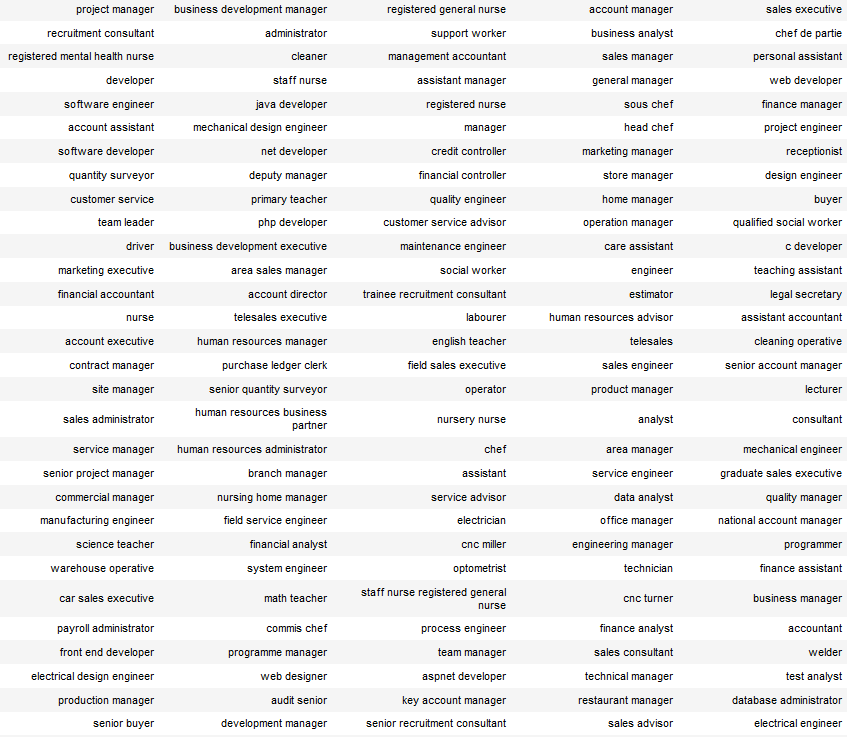


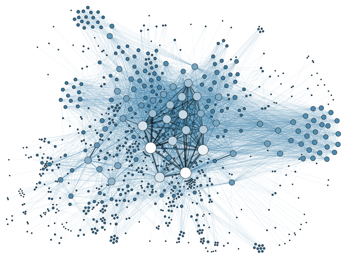
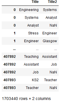
Finding Duplicate Companies with Cliques
jobs
nlp
data
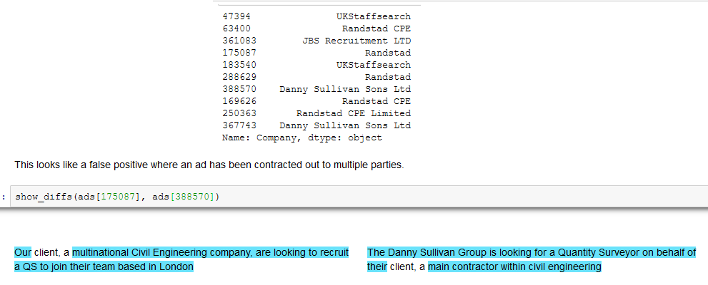
We’ve found pairs of near duplicate texts in 400,000 job ads from the Adzuna Job Salary Predictions Kaggle Competition. When we tried to extracted groups of similar ads by finding connected components in the graph of similar ads. Unfortunately with a low threshold of similarity we ended up with a chain of ads that were each similar, but…


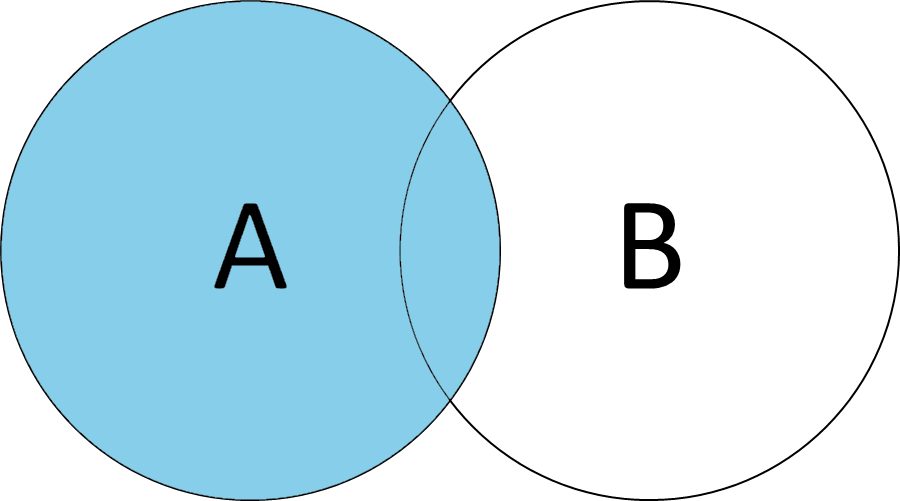
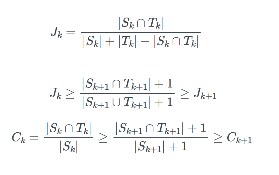
Probability Jaccard
maths
I don’t like Jaccard index for clustering because it doesn’t work well on sets of different sizes. Instead I find the concepts from Association Rule Learning (a.k.a market basket analysis) very useful. It turns out Jaccard Similarity can be written in terms of these concepts so they…


Minhash Sets
jobs
nlp
python
We’ve found pairs of near duplicates texts in the Adzuna Job Salary Predictions Kaggle Competition using Minhash. But many pairs will be part of the same group, in an extreme case there could be a group of 5 job ads with identical texts which produces 10 pairs. Both for interpretability and usability it makes sense to extract…
Searching for Near Duplicates with Minhash
nlp
jobs
python
I’m trying to find near duplicates texts in the Adzuna Job Salary Predictions Kaggle Competition. In the last article I built a collection of MinHashes of the 400,000 job ads in half an hour in a 200MB file. Now I need to efficiently search through these minhashes to find the near duplicates because brute force search…

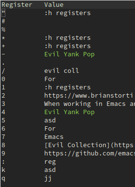
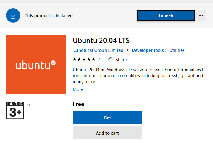
Considering VS Code from Emacs
emacs
I’ve been using Emacs as my primary editor for around 5 years now (after 4 years of Vim). I’m very comfortable in it, having spent a long time configuring my init.el. But once in a while I’m slowed down by some strange issue, so I’m going to put aside my sunk configuration costs and have a look at…
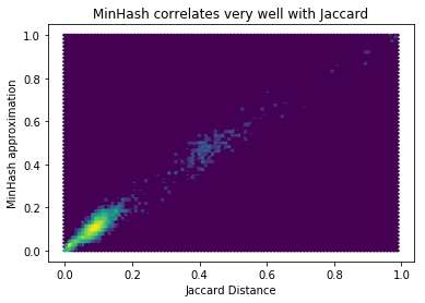
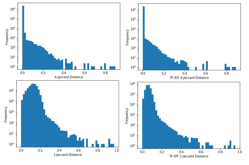
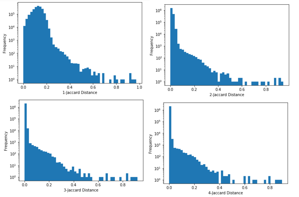
Detecting Near Duplicates with Minhash
nlp
jobs
python
I’m trying to find near duplicates texts in the Adzuna Job Salary Predictions Kaggle Competition. I’ve found that that the Jaccard index on n-grams is effective for finding these. Unfortunately it would take about 8 days to calculate the Jaccard index on all pairs of the 400,000 ads, and take about 640GB of memory to…


Locating Addresses with G-NAF
data
A very useful open dataset the Australian Government provides is the Geocoded National Address File (G-NAF). This is a database mapping addresses to locations. This is really useful for applications that want to provide information or services based on someone’s location. For…
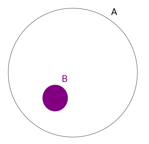
A Mixture of Bernoullis is Bernoulli
maths
Suppose you are analysing email conversion through rates. People either follow the call to action or they don’t, so it’s a Bernoulli Distribution with probability the actual probability a random person will the email. But in actuality your email list will be made up of different groups; for example people who have…


![]()


All of Statistics
data
For anyone who wants to learn Statistics and has a maths or physics I highly recommend Larry Wasserman’s All of Statistics . It covers a wide range of statistics with enough mathematical detail to really understand what’s going on, but not so much that the machinery is overwhelming. What I…

![]()
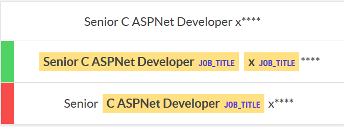

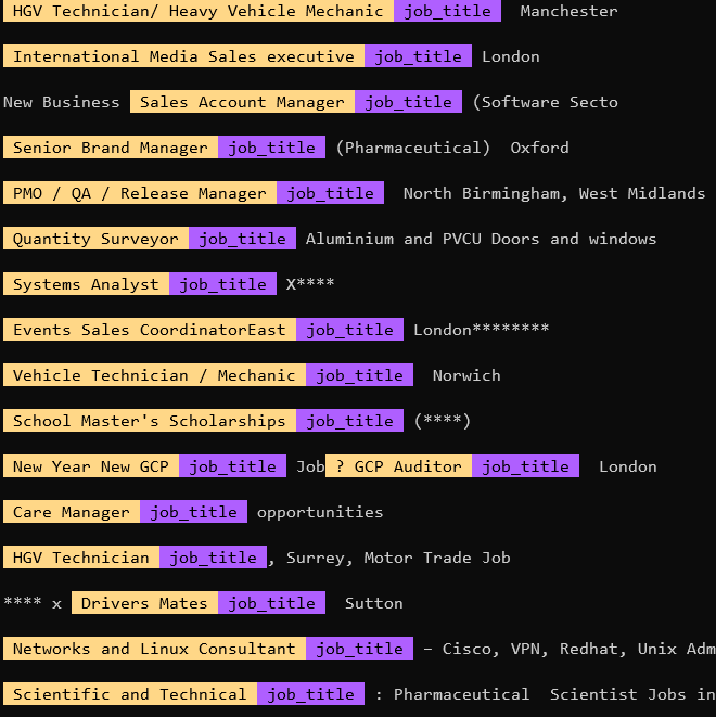
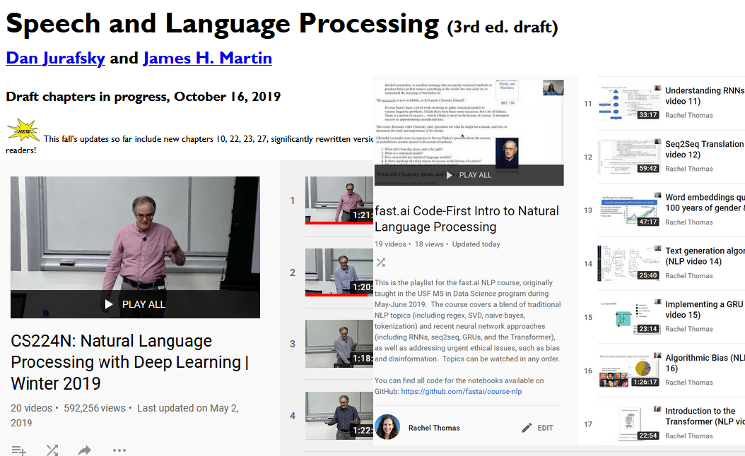
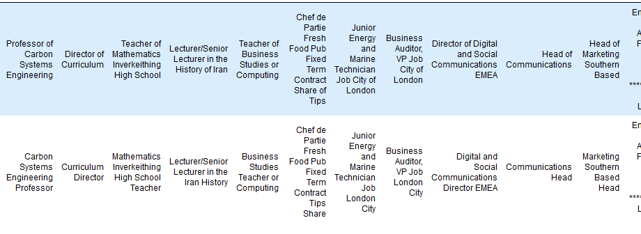
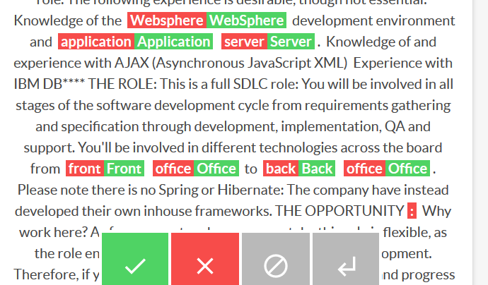
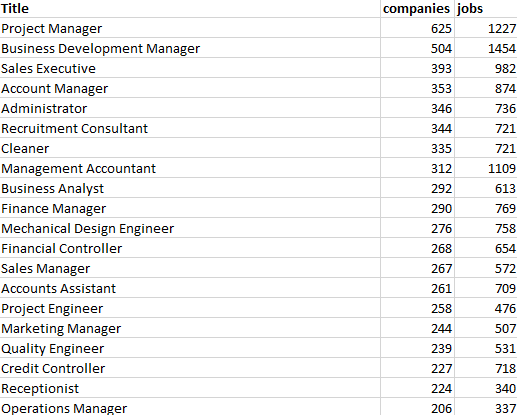
Training a job title NER with Prodigy
nlp
annotation
data
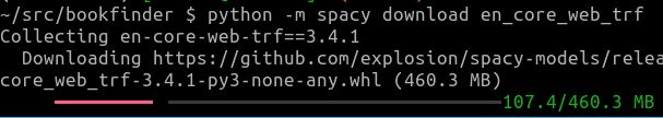
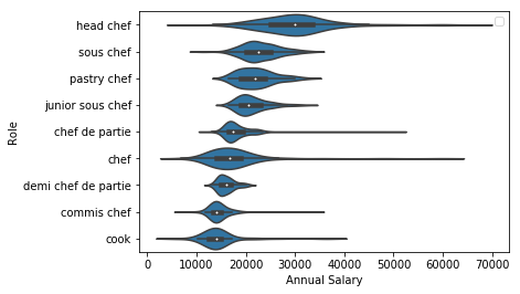
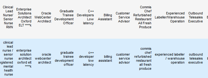
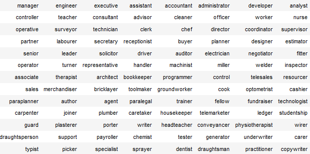
In a couple of hours I trained a reasonable job title Named Entity Recogniser for job ad titles using Prodigy, with over 70% accuracy. While 70% doesn’t sound great it’s a bit ambiguous what a job title is, and getting exactly the bounds of the job title can be a hard…


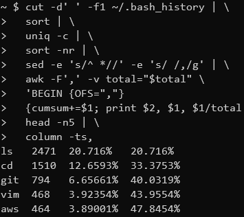
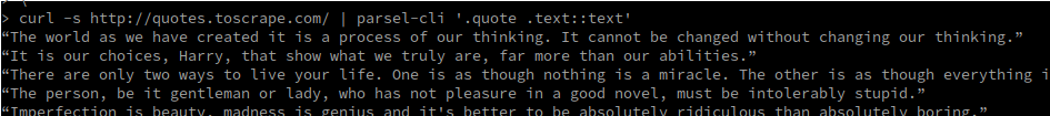
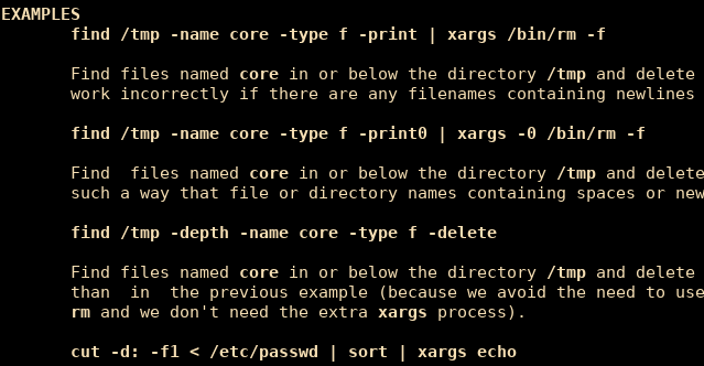
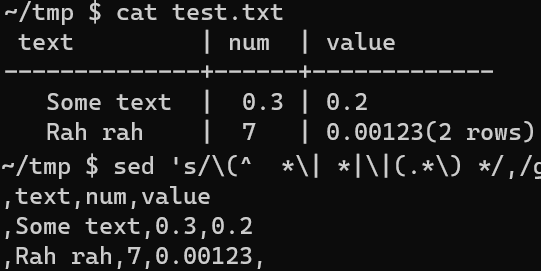
Data Transformations in the Shell
data
linux
There are many great tools for filtering, transforming and aggregating data like SQL, R dplyr and Python Pandas (not to mention Excel). But sometimes when I’m working on a remote server I want to quickly extract some information from a file without switching to one of these…


No matching items