From Bernoulli to Binomial Distributions

Suppose that you flip a fair coin 10 times, how many heads will you get? You’d think it was close to 5, but it might be a bit higher or lower. If you only got 7 heads would you reconsider you assumption the coin is fair? What if you got 70 heads out of 100 flips?

This might seem a bit abstract, but the inverse problem is often very important. Given that 7 out of 10 people convert on a new call to action, can we say it’s more successful than the existing one that converts at 50%? This could be people any proportion, from patients that recover from a medical treatment to people that act on a recommendation. To understand this inverse problem it helps to understand the problem above.

This situation where there are two possible outcomes that occur is called a Bernoulli Trial. For mathematical convenience we label the outcomes 0 and 1 (for “failure” and “success”, but the assignment is arbitrary), and denote the probability of 1 by p. Because there are only two possible outcomes and the total probability is 1, the probability for the outcome 0 is 1-p. Concretely if there’s 30% chance of someone opening an email you sent (p=0.3), then there’s a 70% chance they don’t open it.

Let’s label the outcome of the Bernoulli Trial by the random variable Y. Mathematically we would write the last paragraph as the pair of equations $P(Y=1)=p$ and $P(Y=0)=1-p$. There’s a mathematical trick to write these as a single equation: anything to the power of 1 is itself and anything to the power of 0 is 1 (except sometimes 0). So we can rewrite the equations as $P(Y=1)=p^1(1-p{)}^0$ and $P(Y=0)=p^0(1-p{)}^1$. Then we can combine them as $P(Y=y)=p^y(1-p{)}^{1-y}$ for y either 0 or 1. This bit of arithmetic is a convenient trick.

Any variable Y that satisfies these equations is called Bernoulli distributed. The expectation value of Y is $E(Y)=\sum _{y}P(Y=y)y$, which is p. Similarly the expectation value of $Y^2$ also p; since the square of 0 is 0 and the square of 1 is 1, it’s the same. So the variance of Y is $V(Y)=E(Y^2)-E(Y{)}^2=p-p^2=p(1-p)$.

To interpret this the expectation value is the same as the probability of success, since we coded success as 1 and failure as 0. The variance is a quadratic intersecting the x-axis at 0 and 1. Notice that the variance is 0 if p is 0 or 1; we always get failure or always get success. The variance is maximum when p is 0.5; that’s when we get the biggest spread between heads and tails. When p is one half then the deviation from the mean is plus or minus one half, giving a variance of one quarter.

What if we run multiple independent trials? That is we send multiple emails to different people, or treat multiple different patients, or flip the coin multiple times. We ignore anything else we know and treat them as if they all have the same probability p, since the mixture or Bernouli’s is Bernoulli. How many successes will we get?

Denote each trial by $Y_i$, and the total number of successes in N trials by $Z=\sum _{i=1}^N{Y}_i$. Then the probability can be written as $P(Z=k)=(\genfrac{}{}{0ex}{}{N}{k})p^k(1-p{)}^{N-k}$. This can be seen because the number of ways of getting k successes out of N trials is given by the binomial coefficient $(\genfrac{}{}{0ex}{}{N}{k})$. Then given k successes and N - k failures the probability of that outcome is the product of the probability for each Bernoulli random variable; $p^k(1-p{)}^{N-k}$. A variable with this probability distribution is called Binomally distributed.

Concretely flipping a fair coin 3 times, each time the result is H or T. There is only one way to get 3 heads, HHH, but 3 ways to get 2 heads and 1 tail; THH, HTH, HHT. Since each outcome is equally likely in this example $P(Z=3)=\frac{1}{8}$ and $P(Z=2)=\frac{3}{8}$. You can visualise this with probability squares.

This answers the question of how many heads you would expect if you flip a fair coin 10 times. The probability of getting exactly 5 heads is $(\genfrac{}{}{0ex}{}{5}{10})\frac{1}{2^{10}}$ which is approximately 25%. But the probability of getting exactly 10 heads is $\frac{1}{2^{10}}$ which is about 0.1%. Doing these calculations is straightforward on a computer; but we can get a general idea by looking at the mean and standard deviation.

Trying to calculate the expectation value and variance directly from the probability distribution requires some tricky combinatorics, like you’d find in the excellent book Concrete Mathematics. But the expectation value of a sum of random variables is the sum of the expectation values; so $E(Z)=\sum _{i=1}^{N}E(Y_i)=Np$. This makes intuitive sense; if we send out 100 emails and the open rate is 30%, we expect $100\times 0.3=30$ emails to be opened.

Similarly the variance of a sum of independent random variables is the sum of their variances. So the total variance is $V(Z)=Np(1-p)$, and so the standard deviation increases with the square root of N. The coefficient of variation, that is the standard deviation relative to the mean, is $\sqrt{\frac{1-p}{Np}}$. So quadrupling the sample size halves the spread of the results relative to the mean.

Spread halves as sample size quadruples

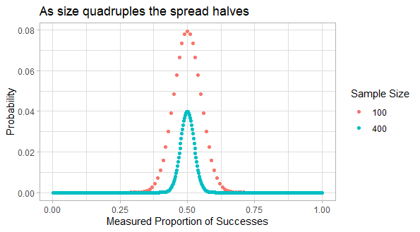
For example there’s a 96% chance of getting 40 to 60 heads in 100 flips of a fair coin; that is 50 ± 20%. If we quadruple the number of flips we just double the range; so there 96% change of getting 180 to 220 heads in 400 flips of a fair coin, that is 200 ± 10%. If we quadruple the number flips again then in 1600 flips there’s a 95% chance of getting 800 ± 5% heads, that is 760 to 840 heads.

In fact as the number of trials increases the binomial distribution gets close to a Normal distribution. It’s a bit complicated exactly when this approximation applies, but it’s slower for more extreme p.