Algorithms for finding the real roots of polynomials
Given an degree n polynomial over the real numbers we are guaranteed there are at most n real roots by the fundamental theorem of algebra; but how do we find them? Here we explore the Vincent-Collins-Akritas algorithm.
It uses Descartes’ rule of signs: given a polynomial \(p(x) = a_n x^n + \cdots + a_1 x + a_0\) the number of real positive roots (counting multiplicites) is bounded above by the number of sign variations in the sequence \((a_n, \ldots, a_1, a_0)\) .
So as an example \(p(x) = x^2 - 1\) has a sequence of coefficients \((1, 0, -1)\) which contains 1 sign change (we ignore zeros), and so has at most one positive root; in fact we know it has exactly one positive root 1. On the other hand the bound is necessary: \(p(x) = (x-(1+i))(x-(1-i))= x^2-2x+2\) has 2 sign changes, but no positive real roots.
Descartes’ theorem tells us about the number of zeros of a degree n polynomial \(p(x)\) on the open interval \((0, \infty)\) ; what if we wanted to know about the number of zeros on some other interval \((u, v)\) ? We could perform a projective transformation \(f(x) = \frac{a x + b}{c x + d}\) ( \(ad - bc \neq 0\) ); in order to still have a polynomial we need to multiply out the denominator to get \(q(x) = (cx+d)^{n} p(\frac{ax +b}{cx+d})\) . The positive zeros of q(x) are the positive zeros of \((cx+d)^n\) and the zeros of p(x) between \(-\frac{b}{a}\) and \(-\frac{d}{c}\) . In particular if we choose a=u, b=v, c=1, d=1 the number of positive zeros of q(x) is precisely the number of zeros of p(x) in the interval \((u, v)\) .
By the rule of signs if q(x) has zero sign variations then p(x) has no root in \((u, v)\) . This leads to our iterative bisection strategy for finding the zeros of a polynomial on an interval. Given a sequence of intervals bisect each interval and find the sign variations of the polynomial projected on each subinterval; if it is zero then discard it, otherwise add it to the next sequence of intervals. This yields a sequence of intervals which may contain zeros of p. However we don’t know which intervals contain no zeros or multiple zeros.
Consider the case of one sign variation; for sufficiently small x, p(x) will have the sign of the terms at the end of the sequence (towards the constant term), and for sufficiently large x, p(x) will have the sign of the leading term. Consequently, since these signs are opposite, by the intermediate value theorem there exists a positive real x such that p(x) is zero. By Descartes’ rule of signs there is at most one real zero; hence there must be exactly one real zero.
Hence we can adjust our algorithm; if there is one sign variation then we add it to a list of definite zeros. However we’re still not sure that the intervals not containing zero will be eliminated; we need a sort-of converse to Descartes’ theorem.
This converse is given by a pair of theorems due to Obreshkoff: Given a degree n polynomial p(x)
- If p(x) has least p complex zeros with arguments in the range \(- \frac{\pi}{n + 2 - p} < \phi < \frac{\pi}{n+2-p}\) then the number of sign variations is bounded above by p.
- If p(x) has at least n-q complex zeros with arguments in range \(\pi - \frac{\pi}{q + 2} \leq \phi \leq \pi + \frac{\pi}{q + 2}\) then the number of sign variations is bounded below by q.
When we translate this by a projective transformation we get a picture like this (taken from Arno Eigenwillig’s thesis)
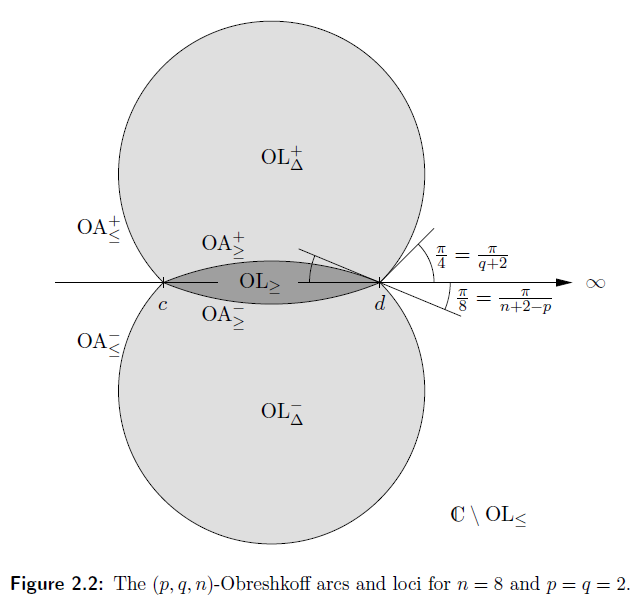
If p(x) has at least p roots in \(OL_{\geq}\) above, then the transformed sign variations are bounded above by p. If p(x) has at most q roots in \(OL_{\leq}\) above then the transformed sign variations are bounded below by q.
Essentially the sign variations can only see zeros “nearby” within these arcs. Since these arcs get smaller as the interval gets smaller it is guaranteed that for sufficiently small intervals (depending on the distance between the roots of the polynomial) the number of sign variations will equal the number of roots.
In particular if all the real roots are simple then the bisection process above will eventually terminate; all intervals will eventually have zero sign variations (in which case there are no roots) or one sign variation (in which case they contain a root).
Hence we have an algorithm for isolating the distinct real roots of a polynomial p(x) over the integers on a bounded interval I.
- Remove all multiple roots by dividing p(x) by the greatest common divisor of p and its derivative.
- The last interval list is {I}, the next interval list is {} and the roots are {}
- Remove each interval from the last interval list, bisect it then add it to the last interval list.
- For each interval in the last interval list calculate the sign variations: if it’s 0 discard it, if it’s 1 add it to the roots, otherwise add it to the next interval list
- If the next interval list is empty return the roots, otherwise set the last interval list to the next interval list, the next interval list to {} and goto 3.
It’s worth noting that transforming the polynomial can be done just with the operations multiply by two, divide by two and add (see On the Various Bisection Methods Derived From Vincents Theorem).
Why just the integers? Polynomials over the rationals can be solved by the same method, by first factoring out the denominators. The real numbers are much more subtle: we can’t calculate the gcd, and worse we can’t even necessarily calculate the sign of a coefficient! (I mean in an algorithmic manner; c.f. Richardson’s Theorem).
One excellent thing about this is the intervals are guaranteed to contain exactly one root; we can then use something like the bisection method to find the zeros to any desired accuracy.
I haven’t been sufficiently precise with my algorithm to analyse it, but there are implementations that use \(O(n^6t^2log^2_nn)\) binary operations on polynomials of degree n on integer t bit coefficients.
There are, of course, other methods of finding all the roots of a real polynomial; but few of them are global and stable like this one. (Though a variation of Newton’s method isn’t a bad candidate, albeit without precise bounds).